Free Statistics
of Irreproducible Research!
Description of Statistical Computation | |||||||||||||||||||||||||||||||||||||||||||||||||||||||||||||||||
|---|---|---|---|---|---|---|---|---|---|---|---|---|---|---|---|---|---|---|---|---|---|---|---|---|---|---|---|---|---|---|---|---|---|---|---|---|---|---|---|---|---|---|---|---|---|---|---|---|---|---|---|---|---|---|---|---|---|---|---|---|---|---|---|---|---|
| Author's title | |||||||||||||||||||||||||||||||||||||||||||||||||||||||||||||||||
| Author | *The author of this computation has been verified* | ||||||||||||||||||||||||||||||||||||||||||||||||||||||||||||||||
| R Software Module | rwasp_edabi.wasp | ||||||||||||||||||||||||||||||||||||||||||||||||||||||||||||||||
| Title produced by software | Bivariate Explorative Data Analysis | ||||||||||||||||||||||||||||||||||||||||||||||||||||||||||||||||
| Date of computation | Tue, 08 Dec 2009 13:18:56 -0700 | ||||||||||||||||||||||||||||||||||||||||||||||||||||||||||||||||
| Cite this page as follows | Statistical Computations at FreeStatistics.org, Office for Research Development and Education, URL https://freestatistics.org/blog/index.php?v=date/2009/Dec/08/t1260303578r1z2jz7anpwaici.htm/, Retrieved Sat, 27 Apr 2024 22:45:39 +0000 | ||||||||||||||||||||||||||||||||||||||||||||||||||||||||||||||||
| Statistical Computations at FreeStatistics.org, Office for Research Development and Education, URL https://freestatistics.org/blog/index.php?pk=64839, Retrieved Sat, 27 Apr 2024 22:45:39 +0000 | |||||||||||||||||||||||||||||||||||||||||||||||||||||||||||||||||
| QR Codes: | |||||||||||||||||||||||||||||||||||||||||||||||||||||||||||||||||
|
| |||||||||||||||||||||||||||||||||||||||||||||||||||||||||||||||||
| Original text written by user: | |||||||||||||||||||||||||||||||||||||||||||||||||||||||||||||||||
| IsPrivate? | No (this computation is public) | ||||||||||||||||||||||||||||||||||||||||||||||||||||||||||||||||
| User-defined keywords | |||||||||||||||||||||||||||||||||||||||||||||||||||||||||||||||||
| Estimated Impact | 143 | ||||||||||||||||||||||||||||||||||||||||||||||||||||||||||||||||
Tree of Dependent Computations | |||||||||||||||||||||||||||||||||||||||||||||||||||||||||||||||||
| Family? (F = Feedback message, R = changed R code, M = changed R Module, P = changed Parameters, D = changed Data) | |||||||||||||||||||||||||||||||||||||||||||||||||||||||||||||||||
| - [Bivariate Explorative Data Analysis] [Workshop 4] [2009-10-29 12:50:48] [1646a2766cb8c4a6f9d3b2fffef409b3] - RM D [Bivariate Explorative Data Analysis] [] [2009-12-08 20:18:56] [d41d8cd98f00b204e9800998ecf8427e] [Current] - D [Bivariate Explorative Data Analysis] [] [2009-12-08 20:28:08] [74be16979710d4c4e7c6647856088456] | |||||||||||||||||||||||||||||||||||||||||||||||||||||||||||||||||
| Feedback Forum | |||||||||||||||||||||||||||||||||||||||||||||||||||||||||||||||||
Post a new message | |||||||||||||||||||||||||||||||||||||||||||||||||||||||||||||||||
Dataset | |||||||||||||||||||||||||||||||||||||||||||||||||||||||||||||||||
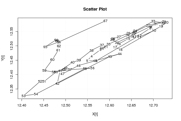
| Dataseries X: | |||||||||||||||||||||||||||||||||||||||||||||||||||||||||||||||||
12,59443229 12,58959203 12,57954817 12,55931771 12,54901675 12,57020869 12,66432942 12,69284735 12,6946864 12,70162827 12,6681701 12,66835592 12,65631033 12,65164269 12,64236113 12,62132305 12,61259053 12,62489811 12,71732618 12,72990728 12,72466404 12,68828581 12,65691575 12,65869166 12,65465471 12,64324312 12,62136596 12,60816206 12,60626722 12,61695969 12,70613556 12,72213354 12,69959747 12,6414816 12,59783091 12,58249678 12,58293936 12,559114 12,52987568 12,51563607 12,4874134 12,48101137 12,60083401 12,62345974 12,56721659 12,52970205 12,4928443 12,49557681 12,50016289 12,47809017 12,45114206 12,44176908 12,4041158 12,43217581 12,54413291 12,56114581 12,50978554 12,47256683 12,45138074 12,46988202 12,48333689 12,48480605 12,48095819 12,47828061 12,45358485 12,48454115 12,59085874 | |||||||||||||||||||||||||||||||||||||||||||||||||||||||||||||||||
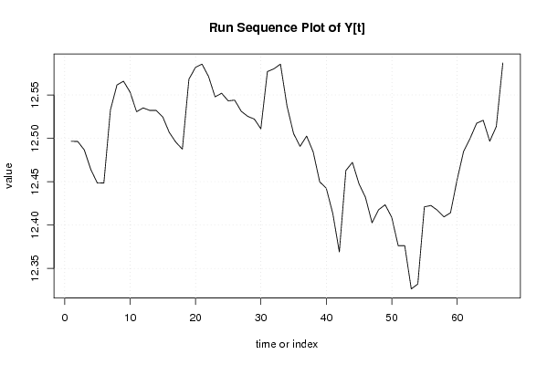
| Dataseries Y: | |||||||||||||||||||||||||||||||||||||||||||||||||||||||||||||||||
12,49654956 12,49637379 12,48664324 12,46405424 12,44840687 12,44850104 12,53273622 12,56147528 12,56584977 12,55335058 12,53064218 12,53507059 12,53223477 12,53214456 12,52466091 12,50673264 12,49552814 12,48745869 12,56813953 12,58171752 12,58553595 12,57136138 12,54780602 12,55198589 12,54322322 12,54400096 12,53118055 12,52531152 12,52216723 12,51102104 12,57695321 12,58013652 12,58553595 12,53719488 12,50553259 12,49072889 12,50259304 12,48437083 12,44979499 12,44253905 12,4133185 12,36892252 12,46286758 12,47224887 12,44769638 12,43178489 12,40255184 12,41756863 12,4233631 12,40917266 12,37615292 12,37617401 12,32631488 12,33199579 12,42091786 12,42252587 12,4170181 12,40941341 12,41415535 12,45201433 12,48491199 12,5000362 12,51739556 12,52074834 12,49661313 12,51353161 12,58693764 | |||||||||||||||||||||||||||||||||||||||||||||||||||||||||||||||||
Tables (Output of Computation) | |||||||||||||||||||||||||||||||||||||||||||||||||||||||||||||||||
| |||||||||||||||||||||||||||||||||||||||||||||||||||||||||||||||||
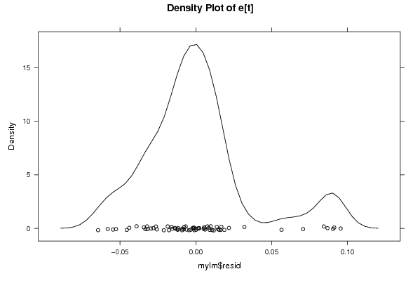
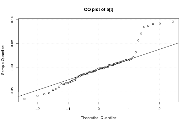
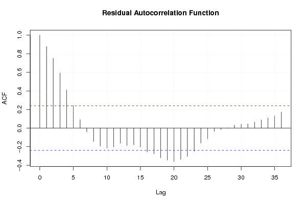
Figures (Output of Computation) | |||||||||||||||||||||||||||||||||||||||||||||||||||||||||||||||||
Input Parameters & R Code | |||||||||||||||||||||||||||||||||||||||||||||||||||||||||||||||||
| Parameters (Session): | |||||||||||||||||||||||||||||||||||||||||||||||||||||||||||||||||
| par1 = 0 ; par2 = 36 ; | |||||||||||||||||||||||||||||||||||||||||||||||||||||||||||||||||
| Parameters (R input): | |||||||||||||||||||||||||||||||||||||||||||||||||||||||||||||||||
| par1 = 0 ; par2 = 36 ; | |||||||||||||||||||||||||||||||||||||||||||||||||||||||||||||||||
| R code (references can be found in the software module): | |||||||||||||||||||||||||||||||||||||||||||||||||||||||||||||||||
par1 <- as.numeric(par1) | |||||||||||||||||||||||||||||||||||||||||||||||||||||||||||||||||