Repository of Reproducible Computations

Free Statistics

of Irreproducible Research!

Author's title

Author

*Unverified author*

R Software Module

rwasp_autocorrelation.wasp

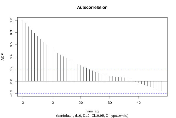
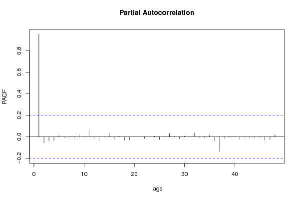
Title produced by software

(Partial) Autocorrelation Function

Date of computation

Tue, 08 Dec 2009 12:46:31 -0700

Cite this page as follows

Statistical Computations at FreeStatistics.org, Office for Research Development and Education, URL https://freestatistics.org/blog/index.php?v=date/2009/Dec/08/t1260301677afknh731uif9pvm.htm/, Retrieved Sun, 28 Apr 2024 02:02:37 +0000

Statistical Computations at FreeStatistics.org, Office for Research Development and Education, URL https://freestatistics.org/blog/index.php?pk=64819, Retrieved Sun, 28 Apr 2024 02:02:37 +0000

QR Codes:

Paste this QR Code to cite your computation.

Original text written by user:

IsPrivate?

No (this computation is public)

User-defined keywords

KDGP2W21

Estimated Impact

142

Family? (F = Feedback message, R = changed R code, M = changed R Module, P = changed Parameters, D = changed Data)

-       [(Partial) Autocorrelation Function] [] [2009-12-08 19:46:31] [d41d8cd98f00b204e9800998ecf8427e] [Current]

Feedback Forum

Post a new message

Dataseries X:

Download CSV

Histogram

Boxplots

Summary of computational transaction
Raw Input	view raw input (R code)
Raw Output	view raw output of R engine
Computing time	1 seconds
R Server	'Gwilym Jenkins' @ 72.249.127.135
R Framework error message	Warning: there are blank lines in the 'Data' field. Please, use NA for missing data - blank lines are simply deleted and are NOT treated as missing values.

\begin{tabular}{lllllllll}
\hline
Summary of computational transaction \tabularnewline
Raw Input & view raw input (R code)  \tabularnewline
Raw Output & view raw output of R engine  \tabularnewline
Computing time & 1 seconds \tabularnewline
R Server & 'Gwilym Jenkins' @ 72.249.127.135 \tabularnewline
R Framework error message & Warning: there are blank lines in the 'Data' field.
Please, use NA for missing data - blank lines are simply
 deleted and are NOT treated as missing values. \tabularnewline
\hline
\end{tabular}
%Source: https://freestatistics.org/blog/index.php?pk=64819&T=0

[TABLE]
[ROW][C]Summary of computational transaction[/C][/ROW]
[ROW][C]Raw Input[/C][C]view raw input (R code) [/C][/ROW]
[ROW][C]Raw Output[/C][C]view raw output of R engine [/C][/ROW]
[ROW][C]Computing time[/C][C]1 seconds[/C][/ROW]
[ROW][C]R Server[/C][C]'Gwilym Jenkins' @ 72.249.127.135[/C][/ROW]
[ROW][C]R Framework error message[/C][C]Warning: there are blank lines in the 'Data' field.
Please, use NA for missing data - blank lines are simply
 deleted and are NOT treated as missing values.[/C][/ROW]
[/TABLE]
Source: https://freestatistics.org/blog/index.php?pk=64819&T=0

Globally Unique Identifier (entire table): ba.freestatistics.org/blog/index.php?pk=64819&T=0

As an alternative you can also use a QR Code:

The GUIDs for individual cells are displayed in the table below:

Summary of computational transaction
Raw Input	view raw input (R code)
Raw Output	view raw output of R engine
Computing time	1 seconds
R Server	'Gwilym Jenkins' @ 72.249.127.135
R Framework error message	Warning: there are blank lines in the 'Data' field. Please, use NA for missing data - blank lines are simply deleted and are NOT treated as missing values.

Autocorrelation Function
Time lag k	ACF(k)	T-STAT	P-value
1	0.950551	9.3135	0
2	0.897991	8.7985	0
3	0.84411	8.2706	0
4	0.78971	7.7375	0
5	0.739112	7.2418	0
6	0.690513	6.7656	0
7	0.644491	6.3147	0
8	0.599698	5.8758	0
9	0.559525	5.4822	0
10	0.521675	5.1113	1e-06
11	0.492334	4.8239	3e-06
12	0.463838	4.5447	8e-06
13	0.434138	4.2537	2.4e-05
14	0.405871	3.9767	6.8e-05
15	0.38187	3.7415	0.000156
16	0.357524	3.503	0.00035
17	0.33523	3.2846	0.000713
18	0.311387	3.051	0.001475
19	0.285445	2.7968	0.003118
20	0.260745	2.5548	0.006099
21	0.237036	2.3225	0.01116
22	0.213879	2.0956	0.019376
23	0.192507	1.8862	0.031147
24	0.173455	1.6995	0.046231
25	0.152971	1.4988	0.068603
26	0.13466	1.3194	0.095089
27	0.120855	1.1841	0.119642
28	0.109058	1.0685	0.143978
29	0.097304	0.9534	0.171396
30	0.087285	0.8552	0.19728
31	0.077743	0.7617	0.224046
32	0.072658	0.7119	0.239128
33	0.067992	0.6662	0.253445
34	0.062745	0.6148	0.270078
35	0.06016	0.5894	0.278473
36	0.053933	0.5284	0.29921
37	0.034409	0.3371	0.368374
38	0.013581	0.1331	0.44721
39	-0.006603	-0.0647	0.474276
40	-0.025708	-0.2519	0.400835
41	-0.045089	-0.4418	0.32982
42	-0.063348	-0.6207	0.268139
43	-0.080629	-0.79	0.215738
44	-0.097023	-0.9506	0.17209
45	-0.111561	-1.0931	0.138549
46	-0.127068	-1.245	0.10808
47	-0.141112	-1.3826	0.084996
48	-0.151761	-1.487	0.070152

\begin{tabular}{lllllllll}
\hline
Autocorrelation Function \tabularnewline
Time lag k & ACF(k) & T-STAT & P-value \tabularnewline
1 & 0.950551 & 9.3135 & 0 \tabularnewline
2 & 0.897991 & 8.7985 & 0 \tabularnewline
3 & 0.84411 & 8.2706 & 0 \tabularnewline
4 & 0.78971 & 7.7375 & 0 \tabularnewline
5 & 0.739112 & 7.2418 & 0 \tabularnewline
6 & 0.690513 & 6.7656 & 0 \tabularnewline
7 & 0.644491 & 6.3147 & 0 \tabularnewline
8 & 0.599698 & 5.8758 & 0 \tabularnewline
9 & 0.559525 & 5.4822 & 0 \tabularnewline
10 & 0.521675 & 5.1113 & 1e-06 \tabularnewline
11 & 0.492334 & 4.8239 & 3e-06 \tabularnewline
12 & 0.463838 & 4.5447 & 8e-06 \tabularnewline
13 & 0.434138 & 4.2537 & 2.4e-05 \tabularnewline
14 & 0.405871 & 3.9767 & 6.8e-05 \tabularnewline
15 & 0.38187 & 3.7415 & 0.000156 \tabularnewline
16 & 0.357524 & 3.503 & 0.00035 \tabularnewline
17 & 0.33523 & 3.2846 & 0.000713 \tabularnewline
18 & 0.311387 & 3.051 & 0.001475 \tabularnewline
19 & 0.285445 & 2.7968 & 0.003118 \tabularnewline
20 & 0.260745 & 2.5548 & 0.006099 \tabularnewline
21 & 0.237036 & 2.3225 & 0.01116 \tabularnewline
22 & 0.213879 & 2.0956 & 0.019376 \tabularnewline
23 & 0.192507 & 1.8862 & 0.031147 \tabularnewline
24 & 0.173455 & 1.6995 & 0.046231 \tabularnewline
25 & 0.152971 & 1.4988 & 0.068603 \tabularnewline
26 & 0.13466 & 1.3194 & 0.095089 \tabularnewline
27 & 0.120855 & 1.1841 & 0.119642 \tabularnewline
28 & 0.109058 & 1.0685 & 0.143978 \tabularnewline
29 & 0.097304 & 0.9534 & 0.171396 \tabularnewline
30 & 0.087285 & 0.8552 & 0.19728 \tabularnewline
31 & 0.077743 & 0.7617 & 0.224046 \tabularnewline
32 & 0.072658 & 0.7119 & 0.239128 \tabularnewline
33 & 0.067992 & 0.6662 & 0.253445 \tabularnewline
34 & 0.062745 & 0.6148 & 0.270078 \tabularnewline
35 & 0.06016 & 0.5894 & 0.278473 \tabularnewline
36 & 0.053933 & 0.5284 & 0.29921 \tabularnewline
37 & 0.034409 & 0.3371 & 0.368374 \tabularnewline
38 & 0.013581 & 0.1331 & 0.44721 \tabularnewline
39 & -0.006603 & -0.0647 & 0.474276 \tabularnewline
40 & -0.025708 & -0.2519 & 0.400835 \tabularnewline
41 & -0.045089 & -0.4418 & 0.32982 \tabularnewline
42 & -0.063348 & -0.6207 & 0.268139 \tabularnewline
43 & -0.080629 & -0.79 & 0.215738 \tabularnewline
44 & -0.097023 & -0.9506 & 0.17209 \tabularnewline
45 & -0.111561 & -1.0931 & 0.138549 \tabularnewline
46 & -0.127068 & -1.245 & 0.10808 \tabularnewline
47 & -0.141112 & -1.3826 & 0.084996 \tabularnewline
48 & -0.151761 & -1.487 & 0.070152 \tabularnewline
\hline
\end{tabular}
%Source: https://freestatistics.org/blog/index.php?pk=64819&T=1

[TABLE]
[ROW][C]Autocorrelation Function[/C][/ROW]
[ROW][C]Time lag k[/C][C]ACF(k)[/C][C]T-STAT[/C][C]P-value[/C][/ROW]
[ROW][C]1[/C][C]0.950551[/C][C]9.3135[/C][C]0[/C][/ROW]
[ROW][C]2[/C][C]0.897991[/C][C]8.7985[/C][C]0[/C][/ROW]
[ROW][C]3[/C][C]0.84411[/C][C]8.2706[/C][C]0[/C][/ROW]
[ROW][C]4[/C][C]0.78971[/C][C]7.7375[/C][C]0[/C][/ROW]
[ROW][C]5[/C][C]0.739112[/C][C]7.2418[/C][C]0[/C][/ROW]
[ROW][C]6[/C][C]0.690513[/C][C]6.7656[/C][C]0[/C][/ROW]
[ROW][C]7[/C][C]0.644491[/C][C]6.3147[/C][C]0[/C][/ROW]
[ROW][C]8[/C][C]0.599698[/C][C]5.8758[/C][C]0[/C][/ROW]
[ROW][C]9[/C][C]0.559525[/C][C]5.4822[/C][C]0[/C][/ROW]
[ROW][C]10[/C][C]0.521675[/C][C]5.1113[/C][C]1e-06[/C][/ROW]
[ROW][C]11[/C][C]0.492334[/C][C]4.8239[/C][C]3e-06[/C][/ROW]
[ROW][C]12[/C][C]0.463838[/C][C]4.5447[/C][C]8e-06[/C][/ROW]
[ROW][C]13[/C][C]0.434138[/C][C]4.2537[/C][C]2.4e-05[/C][/ROW]
[ROW][C]14[/C][C]0.405871[/C][C]3.9767[/C][C]6.8e-05[/C][/ROW]
[ROW][C]15[/C][C]0.38187[/C][C]3.7415[/C][C]0.000156[/C][/ROW]
[ROW][C]16[/C][C]0.357524[/C][C]3.503[/C][C]0.00035[/C][/ROW]
[ROW][C]17[/C][C]0.33523[/C][C]3.2846[/C][C]0.000713[/C][/ROW]
[ROW][C]18[/C][C]0.311387[/C][C]3.051[/C][C]0.001475[/C][/ROW]
[ROW][C]19[/C][C]0.285445[/C][C]2.7968[/C][C]0.003118[/C][/ROW]
[ROW][C]20[/C][C]0.260745[/C][C]2.5548[/C][C]0.006099[/C][/ROW]
[ROW][C]21[/C][C]0.237036[/C][C]2.3225[/C][C]0.01116[/C][/ROW]
[ROW][C]22[/C][C]0.213879[/C][C]2.0956[/C][C]0.019376[/C][/ROW]
[ROW][C]23[/C][C]0.192507[/C][C]1.8862[/C][C]0.031147[/C][/ROW]
[ROW][C]24[/C][C]0.173455[/C][C]1.6995[/C][C]0.046231[/C][/ROW]
[ROW][C]25[/C][C]0.152971[/C][C]1.4988[/C][C]0.068603[/C][/ROW]
[ROW][C]26[/C][C]0.13466[/C][C]1.3194[/C][C]0.095089[/C][/ROW]
[ROW][C]27[/C][C]0.120855[/C][C]1.1841[/C][C]0.119642[/C][/ROW]
[ROW][C]28[/C][C]0.109058[/C][C]1.0685[/C][C]0.143978[/C][/ROW]
[ROW][C]29[/C][C]0.097304[/C][C]0.9534[/C][C]0.171396[/C][/ROW]
[ROW][C]30[/C][C]0.087285[/C][C]0.8552[/C][C]0.19728[/C][/ROW]
[ROW][C]31[/C][C]0.077743[/C][C]0.7617[/C][C]0.224046[/C][/ROW]
[ROW][C]32[/C][C]0.072658[/C][C]0.7119[/C][C]0.239128[/C][/ROW]
[ROW][C]33[/C][C]0.067992[/C][C]0.6662[/C][C]0.253445[/C][/ROW]
[ROW][C]34[/C][C]0.062745[/C][C]0.6148[/C][C]0.270078[/C][/ROW]
[ROW][C]35[/C][C]0.06016[/C][C]0.5894[/C][C]0.278473[/C][/ROW]
[ROW][C]36[/C][C]0.053933[/C][C]0.5284[/C][C]0.29921[/C][/ROW]
[ROW][C]37[/C][C]0.034409[/C][C]0.3371[/C][C]0.368374[/C][/ROW]
[ROW][C]38[/C][C]0.013581[/C][C]0.1331[/C][C]0.44721[/C][/ROW]
[ROW][C]39[/C][C]-0.006603[/C][C]-0.0647[/C][C]0.474276[/C][/ROW]
[ROW][C]40[/C][C]-0.025708[/C][C]-0.2519[/C][C]0.400835[/C][/ROW]
[ROW][C]41[/C][C]-0.045089[/C][C]-0.4418[/C][C]0.32982[/C][/ROW]
[ROW][C]42[/C][C]-0.063348[/C][C]-0.6207[/C][C]0.268139[/C][/ROW]
[ROW][C]43[/C][C]-0.080629[/C][C]-0.79[/C][C]0.215738[/C][/ROW]
[ROW][C]44[/C][C]-0.097023[/C][C]-0.9506[/C][C]0.17209[/C][/ROW]
[ROW][C]45[/C][C]-0.111561[/C][C]-1.0931[/C][C]0.138549[/C][/ROW]
[ROW][C]46[/C][C]-0.127068[/C][C]-1.245[/C][C]0.10808[/C][/ROW]
[ROW][C]47[/C][C]-0.141112[/C][C]-1.3826[/C][C]0.084996[/C][/ROW]
[ROW][C]48[/C][C]-0.151761[/C][C]-1.487[/C][C]0.070152[/C][/ROW]
[/TABLE]
Source: https://freestatistics.org/blog/index.php?pk=64819&T=1

Globally Unique Identifier (entire table): ba.freestatistics.org/blog/index.php?pk=64819&T=1

As an alternative you can also use a QR Code:

The GUIDs for individual cells are displayed in the table below:

Autocorrelation Function
Time lag k	ACF(k)	T-STAT	P-value
1	0.950551	9.3135	0
2	0.897991	8.7985	0
3	0.84411	8.2706	0
4	0.78971	7.7375	0
5	0.739112	7.2418	0
6	0.690513	6.7656	0
7	0.644491	6.3147	0
8	0.599698	5.8758	0
9	0.559525	5.4822	0
10	0.521675	5.1113	1e-06
11	0.492334	4.8239	3e-06
12	0.463838	4.5447	8e-06
13	0.434138	4.2537	2.4e-05
14	0.405871	3.9767	6.8e-05
15	0.38187	3.7415	0.000156
16	0.357524	3.503	0.00035
17	0.33523	3.2846	0.000713
18	0.311387	3.051	0.001475
19	0.285445	2.7968	0.003118
20	0.260745	2.5548	0.006099
21	0.237036	2.3225	0.01116
22	0.213879	2.0956	0.019376
23	0.192507	1.8862	0.031147
24	0.173455	1.6995	0.046231
25	0.152971	1.4988	0.068603
26	0.13466	1.3194	0.095089
27	0.120855	1.1841	0.119642
28	0.109058	1.0685	0.143978
29	0.097304	0.9534	0.171396
30	0.087285	0.8552	0.19728
31	0.077743	0.7617	0.224046
32	0.072658	0.7119	0.239128
33	0.067992	0.6662	0.253445
34	0.062745	0.6148	0.270078
35	0.06016	0.5894	0.278473
36	0.053933	0.5284	0.29921
37	0.034409	0.3371	0.368374
38	0.013581	0.1331	0.44721
39	-0.006603	-0.0647	0.474276
40	-0.025708	-0.2519	0.400835
41	-0.045089	-0.4418	0.32982
42	-0.063348	-0.6207	0.268139
43	-0.080629	-0.79	0.215738
44	-0.097023	-0.9506	0.17209
45	-0.111561	-1.0931	0.138549
46	-0.127068	-1.245	0.10808
47	-0.141112	-1.3826	0.084996
48	-0.151761	-1.487	0.070152

Partial Autocorrelation Function
Time lag k	PACF(k)	T-STAT	P-value
1	0.950551	9.3135	0
2	-0.057614	-0.5645	0.286866
3	-0.040463	-0.3965	0.346324
4	-0.033865	-0.3318	0.370378
5	0.009719	0.0952	0.462166
6	-0.010481	-0.1027	0.459211
7	-0.004082	-0.04	0.484091
8	-0.017868	-0.1751	0.430697
9	0.019766	0.1937	0.423422
10	-0.004251	-0.0416	0.483433
11	0.062511	0.6125	0.270834
12	-0.017663	-0.1731	0.431482
13	-0.032675	-0.3201	0.374776
14	-0.004739	-0.0464	0.481532
15	0.031306	0.3067	0.379856
16	-0.021578	-0.2114	0.416504
17	0.005531	0.0542	0.478446
18	-0.03372	-0.3304	0.370914
19	-0.03054	-0.2992	0.382706
20	-0.001919	-0.0188	0.492521
21	-0.000433	-0.0042	0.498314
22	-0.014432	-0.1414	0.443922
23	-0.001322	-0.013	0.494846
24	0.006646	0.0651	0.47411
25	-0.025425	-0.2491	0.401901
26	0.003114	0.0305	0.487862
27	0.030214	0.296	0.38392
28	0.003518	0.0345	0.486288
29	-0.017196	-0.1685	0.433279
30	0.007853	0.0769	0.469416
31	-0.001236	-0.0121	0.495181
32	0.03649	0.3575	0.360741
33	-0.005975	-0.0585	0.47672
34	-0.010203	-0.1	0.460288
35	0.019815	0.1941	0.423235
36	-0.037359	-0.366	0.35757
37	-0.137384	-1.3461	0.090723
38	-0.016914	-0.1657	0.434363
39	-0.005825	-0.0571	0.477302
40	0.002407	0.0236	0.490615
41	-0.026984	-0.2644	0.396023
42	-0.004323	-0.0424	0.483151
43	-0.010224	-0.1002	0.460207
44	-0.012835	-0.1258	0.450094
45	-0.007302	-0.0715	0.471556
46	-0.032184	-0.3153	0.376596
47	-0.024255	-0.2377	0.406329
48	0.020523	0.2011	0.42053

\begin{tabular}{lllllllll}
\hline
Partial Autocorrelation Function \tabularnewline
Time lag k & PACF(k) & T-STAT & P-value \tabularnewline
1 & 0.950551 & 9.3135 & 0 \tabularnewline
2 & -0.057614 & -0.5645 & 0.286866 \tabularnewline
3 & -0.040463 & -0.3965 & 0.346324 \tabularnewline
4 & -0.033865 & -0.3318 & 0.370378 \tabularnewline
5 & 0.009719 & 0.0952 & 0.462166 \tabularnewline
6 & -0.010481 & -0.1027 & 0.459211 \tabularnewline
7 & -0.004082 & -0.04 & 0.484091 \tabularnewline
8 & -0.017868 & -0.1751 & 0.430697 \tabularnewline
9 & 0.019766 & 0.1937 & 0.423422 \tabularnewline
10 & -0.004251 & -0.0416 & 0.483433 \tabularnewline
11 & 0.062511 & 0.6125 & 0.270834 \tabularnewline
12 & -0.017663 & -0.1731 & 0.431482 \tabularnewline
13 & -0.032675 & -0.3201 & 0.374776 \tabularnewline
14 & -0.004739 & -0.0464 & 0.481532 \tabularnewline
15 & 0.031306 & 0.3067 & 0.379856 \tabularnewline
16 & -0.021578 & -0.2114 & 0.416504 \tabularnewline
17 & 0.005531 & 0.0542 & 0.478446 \tabularnewline
18 & -0.03372 & -0.3304 & 0.370914 \tabularnewline
19 & -0.03054 & -0.2992 & 0.382706 \tabularnewline
20 & -0.001919 & -0.0188 & 0.492521 \tabularnewline
21 & -0.000433 & -0.0042 & 0.498314 \tabularnewline
22 & -0.014432 & -0.1414 & 0.443922 \tabularnewline
23 & -0.001322 & -0.013 & 0.494846 \tabularnewline
24 & 0.006646 & 0.0651 & 0.47411 \tabularnewline
25 & -0.025425 & -0.2491 & 0.401901 \tabularnewline
26 & 0.003114 & 0.0305 & 0.487862 \tabularnewline
27 & 0.030214 & 0.296 & 0.38392 \tabularnewline
28 & 0.003518 & 0.0345 & 0.486288 \tabularnewline
29 & -0.017196 & -0.1685 & 0.433279 \tabularnewline
30 & 0.007853 & 0.0769 & 0.469416 \tabularnewline
31 & -0.001236 & -0.0121 & 0.495181 \tabularnewline
32 & 0.03649 & 0.3575 & 0.360741 \tabularnewline
33 & -0.005975 & -0.0585 & 0.47672 \tabularnewline
34 & -0.010203 & -0.1 & 0.460288 \tabularnewline
35 & 0.019815 & 0.1941 & 0.423235 \tabularnewline
36 & -0.037359 & -0.366 & 0.35757 \tabularnewline
37 & -0.137384 & -1.3461 & 0.090723 \tabularnewline
38 & -0.016914 & -0.1657 & 0.434363 \tabularnewline
39 & -0.005825 & -0.0571 & 0.477302 \tabularnewline
40 & 0.002407 & 0.0236 & 0.490615 \tabularnewline
41 & -0.026984 & -0.2644 & 0.396023 \tabularnewline
42 & -0.004323 & -0.0424 & 0.483151 \tabularnewline
43 & -0.010224 & -0.1002 & 0.460207 \tabularnewline
44 & -0.012835 & -0.1258 & 0.450094 \tabularnewline
45 & -0.007302 & -0.0715 & 0.471556 \tabularnewline
46 & -0.032184 & -0.3153 & 0.376596 \tabularnewline
47 & -0.024255 & -0.2377 & 0.406329 \tabularnewline
48 & 0.020523 & 0.2011 & 0.42053 \tabularnewline
\hline
\end{tabular}
%Source: https://freestatistics.org/blog/index.php?pk=64819&T=2

[TABLE]
[ROW][C]Partial Autocorrelation Function[/C][/ROW]
[ROW][C]Time lag k[/C][C]PACF(k)[/C][C]T-STAT[/C][C]P-value[/C][/ROW]
[ROW][C]1[/C][C]0.950551[/C][C]9.3135[/C][C]0[/C][/ROW]
[ROW][C]2[/C][C]-0.057614[/C][C]-0.5645[/C][C]0.286866[/C][/ROW]
[ROW][C]3[/C][C]-0.040463[/C][C]-0.3965[/C][C]0.346324[/C][/ROW]
[ROW][C]4[/C][C]-0.033865[/C][C]-0.3318[/C][C]0.370378[/C][/ROW]
[ROW][C]5[/C][C]0.009719[/C][C]0.0952[/C][C]0.462166[/C][/ROW]
[ROW][C]6[/C][C]-0.010481[/C][C]-0.1027[/C][C]0.459211[/C][/ROW]
[ROW][C]7[/C][C]-0.004082[/C][C]-0.04[/C][C]0.484091[/C][/ROW]
[ROW][C]8[/C][C]-0.017868[/C][C]-0.1751[/C][C]0.430697[/C][/ROW]
[ROW][C]9[/C][C]0.019766[/C][C]0.1937[/C][C]0.423422[/C][/ROW]
[ROW][C]10[/C][C]-0.004251[/C][C]-0.0416[/C][C]0.483433[/C][/ROW]
[ROW][C]11[/C][C]0.062511[/C][C]0.6125[/C][C]0.270834[/C][/ROW]
[ROW][C]12[/C][C]-0.017663[/C][C]-0.1731[/C][C]0.431482[/C][/ROW]
[ROW][C]13[/C][C]-0.032675[/C][C]-0.3201[/C][C]0.374776[/C][/ROW]
[ROW][C]14[/C][C]-0.004739[/C][C]-0.0464[/C][C]0.481532[/C][/ROW]
[ROW][C]15[/C][C]0.031306[/C][C]0.3067[/C][C]0.379856[/C][/ROW]
[ROW][C]16[/C][C]-0.021578[/C][C]-0.2114[/C][C]0.416504[/C][/ROW]
[ROW][C]17[/C][C]0.005531[/C][C]0.0542[/C][C]0.478446[/C][/ROW]
[ROW][C]18[/C][C]-0.03372[/C][C]-0.3304[/C][C]0.370914[/C][/ROW]
[ROW][C]19[/C][C]-0.03054[/C][C]-0.2992[/C][C]0.382706[/C][/ROW]
[ROW][C]20[/C][C]-0.001919[/C][C]-0.0188[/C][C]0.492521[/C][/ROW]
[ROW][C]21[/C][C]-0.000433[/C][C]-0.0042[/C][C]0.498314[/C][/ROW]
[ROW][C]22[/C][C]-0.014432[/C][C]-0.1414[/C][C]0.443922[/C][/ROW]
[ROW][C]23[/C][C]-0.001322[/C][C]-0.013[/C][C]0.494846[/C][/ROW]
[ROW][C]24[/C][C]0.006646[/C][C]0.0651[/C][C]0.47411[/C][/ROW]
[ROW][C]25[/C][C]-0.025425[/C][C]-0.2491[/C][C]0.401901[/C][/ROW]
[ROW][C]26[/C][C]0.003114[/C][C]0.0305[/C][C]0.487862[/C][/ROW]
[ROW][C]27[/C][C]0.030214[/C][C]0.296[/C][C]0.38392[/C][/ROW]
[ROW][C]28[/C][C]0.003518[/C][C]0.0345[/C][C]0.486288[/C][/ROW]
[ROW][C]29[/C][C]-0.017196[/C][C]-0.1685[/C][C]0.433279[/C][/ROW]
[ROW][C]30[/C][C]0.007853[/C][C]0.0769[/C][C]0.469416[/C][/ROW]
[ROW][C]31[/C][C]-0.001236[/C][C]-0.0121[/C][C]0.495181[/C][/ROW]
[ROW][C]32[/C][C]0.03649[/C][C]0.3575[/C][C]0.360741[/C][/ROW]
[ROW][C]33[/C][C]-0.005975[/C][C]-0.0585[/C][C]0.47672[/C][/ROW]
[ROW][C]34[/C][C]-0.010203[/C][C]-0.1[/C][C]0.460288[/C][/ROW]
[ROW][C]35[/C][C]0.019815[/C][C]0.1941[/C][C]0.423235[/C][/ROW]
[ROW][C]36[/C][C]-0.037359[/C][C]-0.366[/C][C]0.35757[/C][/ROW]
[ROW][C]37[/C][C]-0.137384[/C][C]-1.3461[/C][C]0.090723[/C][/ROW]
[ROW][C]38[/C][C]-0.016914[/C][C]-0.1657[/C][C]0.434363[/C][/ROW]
[ROW][C]39[/C][C]-0.005825[/C][C]-0.0571[/C][C]0.477302[/C][/ROW]
[ROW][C]40[/C][C]0.002407[/C][C]0.0236[/C][C]0.490615[/C][/ROW]
[ROW][C]41[/C][C]-0.026984[/C][C]-0.2644[/C][C]0.396023[/C][/ROW]
[ROW][C]42[/C][C]-0.004323[/C][C]-0.0424[/C][C]0.483151[/C][/ROW]
[ROW][C]43[/C][C]-0.010224[/C][C]-0.1002[/C][C]0.460207[/C][/ROW]
[ROW][C]44[/C][C]-0.012835[/C][C]-0.1258[/C][C]0.450094[/C][/ROW]
[ROW][C]45[/C][C]-0.007302[/C][C]-0.0715[/C][C]0.471556[/C][/ROW]
[ROW][C]46[/C][C]-0.032184[/C][C]-0.3153[/C][C]0.376596[/C][/ROW]
[ROW][C]47[/C][C]-0.024255[/C][C]-0.2377[/C][C]0.406329[/C][/ROW]
[ROW][C]48[/C][C]0.020523[/C][C]0.2011[/C][C]0.42053[/C][/ROW]
[/TABLE]
Source: https://freestatistics.org/blog/index.php?pk=64819&T=2

Globally Unique Identifier (entire table): ba.freestatistics.org/blog/index.php?pk=64819&T=2

As an alternative you can also use a QR Code:

The GUIDs for individual cells are displayed in the table below:

Partial Autocorrelation Function
Time lag k	PACF(k)	T-STAT	P-value
1	0.950551	9.3135	0
2	-0.057614	-0.5645	0.286866
3	-0.040463	-0.3965	0.346324
4	-0.033865	-0.3318	0.370378
5	0.009719	0.0952	0.462166
6	-0.010481	-0.1027	0.459211
7	-0.004082	-0.04	0.484091
8	-0.017868	-0.1751	0.430697
9	0.019766	0.1937	0.423422
10	-0.004251	-0.0416	0.483433
11	0.062511	0.6125	0.270834
12	-0.017663	-0.1731	0.431482
13	-0.032675	-0.3201	0.374776
14	-0.004739	-0.0464	0.481532
15	0.031306	0.3067	0.379856
16	-0.021578	-0.2114	0.416504
17	0.005531	0.0542	0.478446
18	-0.03372	-0.3304	0.370914
19	-0.03054	-0.2992	0.382706
20	-0.001919	-0.0188	0.492521
21	-0.000433	-0.0042	0.498314
22	-0.014432	-0.1414	0.443922
23	-0.001322	-0.013	0.494846
24	0.006646	0.0651	0.47411
25	-0.025425	-0.2491	0.401901
26	0.003114	0.0305	0.487862
27	0.030214	0.296	0.38392
28	0.003518	0.0345	0.486288
29	-0.017196	-0.1685	0.433279
30	0.007853	0.0769	0.469416
31	-0.001236	-0.0121	0.495181
32	0.03649	0.3575	0.360741
33	-0.005975	-0.0585	0.47672
34	-0.010203	-0.1	0.460288
35	0.019815	0.1941	0.423235
36	-0.037359	-0.366	0.35757
37	-0.137384	-1.3461	0.090723
38	-0.016914	-0.1657	0.434363
39	-0.005825	-0.0571	0.477302
40	0.002407	0.0236	0.490615
41	-0.026984	-0.2644	0.396023
42	-0.004323	-0.0424	0.483151
43	-0.010224	-0.1002	0.460207
44	-0.012835	-0.1258	0.450094
45	-0.007302	-0.0715	0.471556
46	-0.032184	-0.3153	0.376596
47	-0.024255	-0.2377	0.406329
48	0.020523	0.2011	0.42053

Figure 1

PNG link

Postscript link

PDF link

Figure 2

PNG link

Postscript link

PDF link

Parameters (Session):

par1 = 48 ; par2 = 1 ; par3 = 0 ; par4 = 0 ; par5 = 12 ; par6 = White Noise ; par7 = 0.95 ;

Parameters (R input):

par1 = 48 ; par2 = 1 ; par3 = 0 ; par4 = 0 ; par5 = 12 ; par6 = White Noise ; par7 = 0.95 ;

R code (references can be found in the software module):

if (par1 == 'Default') {
par1 = 10*log10(length(x))
} else {
par1 <- as.numeric(par1)
}
par2 <- as.numeric(par2)
par3 <- as.numeric(par3)
par4 <- as.numeric(par4)
par5 <- as.numeric(par5)
if (par6 == 'White Noise') par6 <- 'white' else par6 <- 'ma'
par7 <- as.numeric(par7)
if (par2 == 0) {
x <- log(x)
} else {
x <- (x ^ par2 - 1) / par2
}
if (par3 > 0) x <- diff(x,lag=1,difference=par3)
if (par4 > 0) x <- diff(x,lag=par5,difference=par4)
bitmap(file='pic1.png')
racf <- acf(x, par1, main='Autocorrelation', xlab='time lag', ylab='ACF', ci.type=par6, ci=par7, sub=paste('(lambda=',par2,', d=',par3,', D=',par4,', CI=', par7, ', CI type=',par6,')',sep=''))
dev.off()
bitmap(file='pic2.png')
rpacf <- pacf(x,par1,main='Partial Autocorrelation',xlab='lags',ylab='PACF')
dev.off()
(myacf <- c(racf$acf))
(mypacf <- c(rpacf$acf))
lengthx <- length(x)
sqrtn <- sqrt(lengthx)
load(file='createtable')
a<-table.start()
a<-table.row.start(a)
a<-table.element(a,'Autocorrelation Function',4,TRUE)
a<-table.row.end(a)
a<-table.row.start(a)
a<-table.element(a,'Time lag k',header=TRUE)
a<-table.element(a,hyperlink('basics.htm','ACF(k)','click here for more information about the Autocorrelation Function'),header=TRUE)
a<-table.element(a,'T-STAT',header=TRUE)
a<-table.element(a,'P-value',header=TRUE)
a<-table.row.end(a)
for (i in 2:(par1+1)) {
a<-table.row.start(a)
a<-table.element(a,i-1,header=TRUE)
a<-table.element(a,round(myacf[i],6))
mytstat <- myacf[i]*sqrtn
a<-table.element(a,round(mytstat,4))
a<-table.element(a,round(1-pt(abs(mytstat),lengthx),6))
a<-table.row.end(a)
}
a<-table.end(a)
table.save(a,file='mytable.tab')
a<-table.start()
a<-table.row.start(a)
a<-table.element(a,'Partial Autocorrelation Function',4,TRUE)
a<-table.row.end(a)
a<-table.row.start(a)
a<-table.element(a,'Time lag k',header=TRUE)
a<-table.element(a,hyperlink('basics.htm','PACF(k)','click here for more information about the Partial Autocorrelation Function'),header=TRUE)
a<-table.element(a,'T-STAT',header=TRUE)
a<-table.element(a,'P-value',header=TRUE)
a<-table.row.end(a)
for (i in 1:par1) {
a<-table.row.start(a)
a<-table.element(a,i,header=TRUE)
a<-table.element(a,round(mypacf[i],6))
mytstat <- mypacf[i]*sqrtn
a<-table.element(a,round(mytstat,4))
a<-table.element(a,round(1-pt(abs(mytstat),lengthx),6))
a<-table.row.end(a)
}
a<-table.end(a)
table.save(a,file='mytable1.tab')

Free Statistics

Description of Statistical Computation

Tree of Dependent Computations

Dataset

Tables (Output of Computation)

Figures (Output of Computation)

Input Parameters & R Code