Repository of Reproducible Computations

Free Statistics

of Irreproducible Research!

Author's title

Author

*Unverified author*

R Software Module

rwasp_autocorrelation.wasp

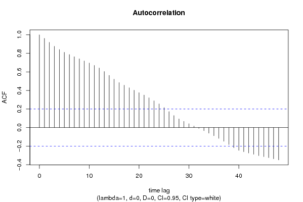
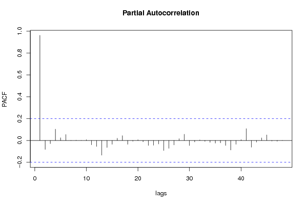
Title produced by software

(Partial) Autocorrelation Function

Date of computation

Tue, 08 Dec 2009 11:25:43 -0700

Cite this page as follows

Statistical Computations at FreeStatistics.org, Office for Research Development and Education, URL https://freestatistics.org/blog/index.php?v=date/2009/Dec/08/t1260296803pzs7ssaiohg3w4y.htm/, Retrieved Sun, 28 Apr 2024 13:09:45 +0000

Statistical Computations at FreeStatistics.org, Office for Research Development and Education, URL https://freestatistics.org/blog/index.php?pk=64767, Retrieved Sun, 28 Apr 2024 13:09:45 +0000

QR Codes:

Paste this QR Code to cite your computation.

Original text written by user:

IsPrivate?

No (this computation is public)

User-defined keywords

KDGP2W12

Estimated Impact

102

Family? (F = Feedback message, R = changed R code, M = changed R Module, P = changed Parameters, D = changed Data)

-       [(Partial) Autocorrelation Function] [Opdracht 6 bis oe...] [2009-12-08 18:25:43] [243e584c296eec1181ddc9ac4f09d2dd] [Current]

Feedback Forum

Post a new message

Dataseries X:

Download CSV

Histogram

Boxplots

Summary of computational transaction
Raw Input	view raw input (R code)
Raw Output	view raw output of R engine
Computing time	1 seconds
R Server	'Gwilym Jenkins' @ 72.249.127.135

\begin{tabular}{lllllllll}
\hline
Summary of computational transaction \tabularnewline
Raw Input & view raw input (R code)  \tabularnewline
Raw Output & view raw output of R engine  \tabularnewline
Computing time & 1 seconds \tabularnewline
R Server & 'Gwilym Jenkins' @ 72.249.127.135 \tabularnewline
\hline
\end{tabular}
%Source: https://freestatistics.org/blog/index.php?pk=64767&T=0

[TABLE]
[ROW][C]Summary of computational transaction[/C][/ROW]
[ROW][C]Raw Input[/C][C]view raw input (R code) [/C][/ROW]
[ROW][C]Raw Output[/C][C]view raw output of R engine [/C][/ROW]
[ROW][C]Computing time[/C][C]1 seconds[/C][/ROW]
[ROW][C]R Server[/C][C]'Gwilym Jenkins' @ 72.249.127.135[/C][/ROW]
[/TABLE]
Source: https://freestatistics.org/blog/index.php?pk=64767&T=0

Globally Unique Identifier (entire table): ba.freestatistics.org/blog/index.php?pk=64767&T=0

As an alternative you can also use a QR Code:

The GUIDs for individual cells are displayed in the table below:

Summary of computational transaction
Raw Input	view raw input (R code)
Raw Output	view raw output of R engine
Computing time	1 seconds
R Server	'Gwilym Jenkins' @ 72.249.127.135

Autocorrelation Function
Time lag k	ACF(k)	T-STAT	P-value
1	0.962064	9.4263	0
2	0.919425	9.0085	0
3	0.875957	8.5826	0
4	0.841712	8.2471	0
5	0.811764	7.9536	0
6	0.787716	7.718	0
7	0.764274	7.4883	0
8	0.741386	7.2641	0
9	0.718138	7.0363	0
10	0.69576	6.817	0
11	0.670905	6.5735	0
12	0.6426	6.2962	0
13	0.604846	5.9263	0
14	0.563429	5.5205	0
15	0.521571	5.1103	1e-06
16	0.485603	4.7579	3e-06
17	0.456934	4.477	1e-05
18	0.429666	4.2098	2.9e-05
19	0.403146	3.95	7.5e-05
20	0.377182	3.6956	0.000182
21	0.350767	3.4368	0.000436
22	0.321511	3.1501	0.001088
23	0.289516	2.8367	0.002781
24	0.255664	2.505	0.006965
25	0.215999	2.1164	0.018451
26	0.172943	1.6945	0.046707
27	0.130186	1.2756	0.102596
28	0.093992	0.9209	0.179699
29	0.067458	0.661	0.255113
30	0.04194	0.4109	0.341021
31	0.017049	0.167	0.433843
32	-0.008027	-0.0786	0.468739
33	-0.033482	-0.3281	0.371791
34	-0.060092	-0.5888	0.278695
35	-0.087875	-0.861	0.195692
36	-0.11651	-1.1416	0.128238
37	-0.147484	-1.445	0.075851
38	-0.182578	-1.7889	0.038393
39	-0.216911	-2.1253	0.018065
40	-0.245537	-2.4058	0.009027
41	-0.259823	-2.5457	0.006248
42	-0.273945	-2.6841	0.004283
43	-0.287499	-2.8169	0.002943
44	-0.301722	-2.9563	0.001959
45	-0.312774	-3.0645	0.001415
46	-0.324397	-3.1784	0.000997
47	-0.335976	-3.2919	0.000697
48	-0.348047	-3.4102	0.000476

\begin{tabular}{lllllllll}
\hline
Autocorrelation Function \tabularnewline
Time lag k & ACF(k) & T-STAT & P-value \tabularnewline
1 & 0.962064 & 9.4263 & 0 \tabularnewline
2 & 0.919425 & 9.0085 & 0 \tabularnewline
3 & 0.875957 & 8.5826 & 0 \tabularnewline
4 & 0.841712 & 8.2471 & 0 \tabularnewline
5 & 0.811764 & 7.9536 & 0 \tabularnewline
6 & 0.787716 & 7.718 & 0 \tabularnewline
7 & 0.764274 & 7.4883 & 0 \tabularnewline
8 & 0.741386 & 7.2641 & 0 \tabularnewline
9 & 0.718138 & 7.0363 & 0 \tabularnewline
10 & 0.69576 & 6.817 & 0 \tabularnewline
11 & 0.670905 & 6.5735 & 0 \tabularnewline
12 & 0.6426 & 6.2962 & 0 \tabularnewline
13 & 0.604846 & 5.9263 & 0 \tabularnewline
14 & 0.563429 & 5.5205 & 0 \tabularnewline
15 & 0.521571 & 5.1103 & 1e-06 \tabularnewline
16 & 0.485603 & 4.7579 & 3e-06 \tabularnewline
17 & 0.456934 & 4.477 & 1e-05 \tabularnewline
18 & 0.429666 & 4.2098 & 2.9e-05 \tabularnewline
19 & 0.403146 & 3.95 & 7.5e-05 \tabularnewline
20 & 0.377182 & 3.6956 & 0.000182 \tabularnewline
21 & 0.350767 & 3.4368 & 0.000436 \tabularnewline
22 & 0.321511 & 3.1501 & 0.001088 \tabularnewline
23 & 0.289516 & 2.8367 & 0.002781 \tabularnewline
24 & 0.255664 & 2.505 & 0.006965 \tabularnewline
25 & 0.215999 & 2.1164 & 0.018451 \tabularnewline
26 & 0.172943 & 1.6945 & 0.046707 \tabularnewline
27 & 0.130186 & 1.2756 & 0.102596 \tabularnewline
28 & 0.093992 & 0.9209 & 0.179699 \tabularnewline
29 & 0.067458 & 0.661 & 0.255113 \tabularnewline
30 & 0.04194 & 0.4109 & 0.341021 \tabularnewline
31 & 0.017049 & 0.167 & 0.433843 \tabularnewline
32 & -0.008027 & -0.0786 & 0.468739 \tabularnewline
33 & -0.033482 & -0.3281 & 0.371791 \tabularnewline
34 & -0.060092 & -0.5888 & 0.278695 \tabularnewline
35 & -0.087875 & -0.861 & 0.195692 \tabularnewline
36 & -0.11651 & -1.1416 & 0.128238 \tabularnewline
37 & -0.147484 & -1.445 & 0.075851 \tabularnewline
38 & -0.182578 & -1.7889 & 0.038393 \tabularnewline
39 & -0.216911 & -2.1253 & 0.018065 \tabularnewline
40 & -0.245537 & -2.4058 & 0.009027 \tabularnewline
41 & -0.259823 & -2.5457 & 0.006248 \tabularnewline
42 & -0.273945 & -2.6841 & 0.004283 \tabularnewline
43 & -0.287499 & -2.8169 & 0.002943 \tabularnewline
44 & -0.301722 & -2.9563 & 0.001959 \tabularnewline
45 & -0.312774 & -3.0645 & 0.001415 \tabularnewline
46 & -0.324397 & -3.1784 & 0.000997 \tabularnewline
47 & -0.335976 & -3.2919 & 0.000697 \tabularnewline
48 & -0.348047 & -3.4102 & 0.000476 \tabularnewline
\hline
\end{tabular}
%Source: https://freestatistics.org/blog/index.php?pk=64767&T=1

[TABLE]
[ROW][C]Autocorrelation Function[/C][/ROW]
[ROW][C]Time lag k[/C][C]ACF(k)[/C][C]T-STAT[/C][C]P-value[/C][/ROW]
[ROW][C]1[/C][C]0.962064[/C][C]9.4263[/C][C]0[/C][/ROW]
[ROW][C]2[/C][C]0.919425[/C][C]9.0085[/C][C]0[/C][/ROW]
[ROW][C]3[/C][C]0.875957[/C][C]8.5826[/C][C]0[/C][/ROW]
[ROW][C]4[/C][C]0.841712[/C][C]8.2471[/C][C]0[/C][/ROW]
[ROW][C]5[/C][C]0.811764[/C][C]7.9536[/C][C]0[/C][/ROW]
[ROW][C]6[/C][C]0.787716[/C][C]7.718[/C][C]0[/C][/ROW]
[ROW][C]7[/C][C]0.764274[/C][C]7.4883[/C][C]0[/C][/ROW]
[ROW][C]8[/C][C]0.741386[/C][C]7.2641[/C][C]0[/C][/ROW]
[ROW][C]9[/C][C]0.718138[/C][C]7.0363[/C][C]0[/C][/ROW]
[ROW][C]10[/C][C]0.69576[/C][C]6.817[/C][C]0[/C][/ROW]
[ROW][C]11[/C][C]0.670905[/C][C]6.5735[/C][C]0[/C][/ROW]
[ROW][C]12[/C][C]0.6426[/C][C]6.2962[/C][C]0[/C][/ROW]
[ROW][C]13[/C][C]0.604846[/C][C]5.9263[/C][C]0[/C][/ROW]
[ROW][C]14[/C][C]0.563429[/C][C]5.5205[/C][C]0[/C][/ROW]
[ROW][C]15[/C][C]0.521571[/C][C]5.1103[/C][C]1e-06[/C][/ROW]
[ROW][C]16[/C][C]0.485603[/C][C]4.7579[/C][C]3e-06[/C][/ROW]
[ROW][C]17[/C][C]0.456934[/C][C]4.477[/C][C]1e-05[/C][/ROW]
[ROW][C]18[/C][C]0.429666[/C][C]4.2098[/C][C]2.9e-05[/C][/ROW]
[ROW][C]19[/C][C]0.403146[/C][C]3.95[/C][C]7.5e-05[/C][/ROW]
[ROW][C]20[/C][C]0.377182[/C][C]3.6956[/C][C]0.000182[/C][/ROW]
[ROW][C]21[/C][C]0.350767[/C][C]3.4368[/C][C]0.000436[/C][/ROW]
[ROW][C]22[/C][C]0.321511[/C][C]3.1501[/C][C]0.001088[/C][/ROW]
[ROW][C]23[/C][C]0.289516[/C][C]2.8367[/C][C]0.002781[/C][/ROW]
[ROW][C]24[/C][C]0.255664[/C][C]2.505[/C][C]0.006965[/C][/ROW]
[ROW][C]25[/C][C]0.215999[/C][C]2.1164[/C][C]0.018451[/C][/ROW]
[ROW][C]26[/C][C]0.172943[/C][C]1.6945[/C][C]0.046707[/C][/ROW]
[ROW][C]27[/C][C]0.130186[/C][C]1.2756[/C][C]0.102596[/C][/ROW]
[ROW][C]28[/C][C]0.093992[/C][C]0.9209[/C][C]0.179699[/C][/ROW]
[ROW][C]29[/C][C]0.067458[/C][C]0.661[/C][C]0.255113[/C][/ROW]
[ROW][C]30[/C][C]0.04194[/C][C]0.4109[/C][C]0.341021[/C][/ROW]
[ROW][C]31[/C][C]0.017049[/C][C]0.167[/C][C]0.433843[/C][/ROW]
[ROW][C]32[/C][C]-0.008027[/C][C]-0.0786[/C][C]0.468739[/C][/ROW]
[ROW][C]33[/C][C]-0.033482[/C][C]-0.3281[/C][C]0.371791[/C][/ROW]
[ROW][C]34[/C][C]-0.060092[/C][C]-0.5888[/C][C]0.278695[/C][/ROW]
[ROW][C]35[/C][C]-0.087875[/C][C]-0.861[/C][C]0.195692[/C][/ROW]
[ROW][C]36[/C][C]-0.11651[/C][C]-1.1416[/C][C]0.128238[/C][/ROW]
[ROW][C]37[/C][C]-0.147484[/C][C]-1.445[/C][C]0.075851[/C][/ROW]
[ROW][C]38[/C][C]-0.182578[/C][C]-1.7889[/C][C]0.038393[/C][/ROW]
[ROW][C]39[/C][C]-0.216911[/C][C]-2.1253[/C][C]0.018065[/C][/ROW]
[ROW][C]40[/C][C]-0.245537[/C][C]-2.4058[/C][C]0.009027[/C][/ROW]
[ROW][C]41[/C][C]-0.259823[/C][C]-2.5457[/C][C]0.006248[/C][/ROW]
[ROW][C]42[/C][C]-0.273945[/C][C]-2.6841[/C][C]0.004283[/C][/ROW]
[ROW][C]43[/C][C]-0.287499[/C][C]-2.8169[/C][C]0.002943[/C][/ROW]
[ROW][C]44[/C][C]-0.301722[/C][C]-2.9563[/C][C]0.001959[/C][/ROW]
[ROW][C]45[/C][C]-0.312774[/C][C]-3.0645[/C][C]0.001415[/C][/ROW]
[ROW][C]46[/C][C]-0.324397[/C][C]-3.1784[/C][C]0.000997[/C][/ROW]
[ROW][C]47[/C][C]-0.335976[/C][C]-3.2919[/C][C]0.000697[/C][/ROW]
[ROW][C]48[/C][C]-0.348047[/C][C]-3.4102[/C][C]0.000476[/C][/ROW]
[/TABLE]
Source: https://freestatistics.org/blog/index.php?pk=64767&T=1

Globally Unique Identifier (entire table): ba.freestatistics.org/blog/index.php?pk=64767&T=1

As an alternative you can also use a QR Code:

The GUIDs for individual cells are displayed in the table below:

Autocorrelation Function
Time lag k	ACF(k)	T-STAT	P-value
1	0.962064	9.4263	0
2	0.919425	9.0085	0
3	0.875957	8.5826	0
4	0.841712	8.2471	0
5	0.811764	7.9536	0
6	0.787716	7.718	0
7	0.764274	7.4883	0
8	0.741386	7.2641	0
9	0.718138	7.0363	0
10	0.69576	6.817	0
11	0.670905	6.5735	0
12	0.6426	6.2962	0
13	0.604846	5.9263	0
14	0.563429	5.5205	0
15	0.521571	5.1103	1e-06
16	0.485603	4.7579	3e-06
17	0.456934	4.477	1e-05
18	0.429666	4.2098	2.9e-05
19	0.403146	3.95	7.5e-05
20	0.377182	3.6956	0.000182
21	0.350767	3.4368	0.000436
22	0.321511	3.1501	0.001088
23	0.289516	2.8367	0.002781
24	0.255664	2.505	0.006965
25	0.215999	2.1164	0.018451
26	0.172943	1.6945	0.046707
27	0.130186	1.2756	0.102596
28	0.093992	0.9209	0.179699
29	0.067458	0.661	0.255113
30	0.04194	0.4109	0.341021
31	0.017049	0.167	0.433843
32	-0.008027	-0.0786	0.468739
33	-0.033482	-0.3281	0.371791
34	-0.060092	-0.5888	0.278695
35	-0.087875	-0.861	0.195692
36	-0.11651	-1.1416	0.128238
37	-0.147484	-1.445	0.075851
38	-0.182578	-1.7889	0.038393
39	-0.216911	-2.1253	0.018065
40	-0.245537	-2.4058	0.009027
41	-0.259823	-2.5457	0.006248
42	-0.273945	-2.6841	0.004283
43	-0.287499	-2.8169	0.002943
44	-0.301722	-2.9563	0.001959
45	-0.312774	-3.0645	0.001415
46	-0.324397	-3.1784	0.000997
47	-0.335976	-3.2919	0.000697
48	-0.348047	-3.4102	0.000476

Partial Autocorrelation Function
Time lag k	PACF(k)	T-STAT	P-value
1	0.962064	9.4263	0
2	-0.082517	-0.8085	0.210402
3	-0.029648	-0.2905	0.386035
4	0.102773	1.007	0.158242
5	0.024709	0.2421	0.404609
6	0.054112	0.5302	0.298602
7	-0.001542	-0.0151	0.493988
8	0.001944	0.019	0.492421
9	-0.000363	-0.0036	0.498585
10	0.006625	0.0649	0.474188
11	-0.040264	-0.3945	0.347043
12	-0.05558	-0.5446	0.293656
13	-0.135361	-1.3263	0.093951
14	-0.064552	-0.6325	0.264289
15	-0.035629	-0.3491	0.363892
16	0.019861	0.1946	0.42306
17	0.043533	0.4265	0.335337
18	-0.035188	-0.3448	0.36551
19	-0.007501	-0.0735	0.470783
20	0.006361	0.0623	0.475216
21	-0.012407	-0.1216	0.451749
22	-0.045702	-0.4478	0.327657
23	-0.044016	-0.4313	0.333619
24	-0.032498	-0.3184	0.375433
25	-0.092285	-0.9042	0.184076
26	-0.072512	-0.7105	0.239569
27	-0.041386	-0.4055	0.343008
28	0.016366	0.1604	0.43647
29	0.056537	0.554	0.29045
30	-0.046696	-0.4575	0.324164
31	-0.01401	-0.1373	0.445551
32	0.004337	0.0425	0.483095
33	-0.008499	-0.0833	0.466904
34	-0.017659	-0.173	0.431499
35	-0.024811	-0.2431	0.404225
36	-0.022494	-0.2204	0.413014
37	-0.046205	-0.4527	0.325889
38	-0.08769	-0.8592	0.196189
39	-0.035235	-0.3452	0.365338
40	0.006829	0.0669	0.473397
41	0.10791	1.0573	0.146513
42	-0.062122	-0.6087	0.272091
43	-0.015458	-0.1515	0.439966
44	0.02323	0.2276	0.410217
45	0.051008	0.4998	0.309188
46	-0.005759	-0.0564	0.477558
47	-0.007201	-0.0706	0.471948
48	-0.000838	-0.0082	0.496734

\begin{tabular}{lllllllll}
\hline
Partial Autocorrelation Function \tabularnewline
Time lag k & PACF(k) & T-STAT & P-value \tabularnewline
1 & 0.962064 & 9.4263 & 0 \tabularnewline
2 & -0.082517 & -0.8085 & 0.210402 \tabularnewline
3 & -0.029648 & -0.2905 & 0.386035 \tabularnewline
4 & 0.102773 & 1.007 & 0.158242 \tabularnewline
5 & 0.024709 & 0.2421 & 0.404609 \tabularnewline
6 & 0.054112 & 0.5302 & 0.298602 \tabularnewline
7 & -0.001542 & -0.0151 & 0.493988 \tabularnewline
8 & 0.001944 & 0.019 & 0.492421 \tabularnewline
9 & -0.000363 & -0.0036 & 0.498585 \tabularnewline
10 & 0.006625 & 0.0649 & 0.474188 \tabularnewline
11 & -0.040264 & -0.3945 & 0.347043 \tabularnewline
12 & -0.05558 & -0.5446 & 0.293656 \tabularnewline
13 & -0.135361 & -1.3263 & 0.093951 \tabularnewline
14 & -0.064552 & -0.6325 & 0.264289 \tabularnewline
15 & -0.035629 & -0.3491 & 0.363892 \tabularnewline
16 & 0.019861 & 0.1946 & 0.42306 \tabularnewline
17 & 0.043533 & 0.4265 & 0.335337 \tabularnewline
18 & -0.035188 & -0.3448 & 0.36551 \tabularnewline
19 & -0.007501 & -0.0735 & 0.470783 \tabularnewline
20 & 0.006361 & 0.0623 & 0.475216 \tabularnewline
21 & -0.012407 & -0.1216 & 0.451749 \tabularnewline
22 & -0.045702 & -0.4478 & 0.327657 \tabularnewline
23 & -0.044016 & -0.4313 & 0.333619 \tabularnewline
24 & -0.032498 & -0.3184 & 0.375433 \tabularnewline
25 & -0.092285 & -0.9042 & 0.184076 \tabularnewline
26 & -0.072512 & -0.7105 & 0.239569 \tabularnewline
27 & -0.041386 & -0.4055 & 0.343008 \tabularnewline
28 & 0.016366 & 0.1604 & 0.43647 \tabularnewline
29 & 0.056537 & 0.554 & 0.29045 \tabularnewline
30 & -0.046696 & -0.4575 & 0.324164 \tabularnewline
31 & -0.01401 & -0.1373 & 0.445551 \tabularnewline
32 & 0.004337 & 0.0425 & 0.483095 \tabularnewline
33 & -0.008499 & -0.0833 & 0.466904 \tabularnewline
34 & -0.017659 & -0.173 & 0.431499 \tabularnewline
35 & -0.024811 & -0.2431 & 0.404225 \tabularnewline
36 & -0.022494 & -0.2204 & 0.413014 \tabularnewline
37 & -0.046205 & -0.4527 & 0.325889 \tabularnewline
38 & -0.08769 & -0.8592 & 0.196189 \tabularnewline
39 & -0.035235 & -0.3452 & 0.365338 \tabularnewline
40 & 0.006829 & 0.0669 & 0.473397 \tabularnewline
41 & 0.10791 & 1.0573 & 0.146513 \tabularnewline
42 & -0.062122 & -0.6087 & 0.272091 \tabularnewline
43 & -0.015458 & -0.1515 & 0.439966 \tabularnewline
44 & 0.02323 & 0.2276 & 0.410217 \tabularnewline
45 & 0.051008 & 0.4998 & 0.309188 \tabularnewline
46 & -0.005759 & -0.0564 & 0.477558 \tabularnewline
47 & -0.007201 & -0.0706 & 0.471948 \tabularnewline
48 & -0.000838 & -0.0082 & 0.496734 \tabularnewline
\hline
\end{tabular}
%Source: https://freestatistics.org/blog/index.php?pk=64767&T=2

[TABLE]
[ROW][C]Partial Autocorrelation Function[/C][/ROW]
[ROW][C]Time lag k[/C][C]PACF(k)[/C][C]T-STAT[/C][C]P-value[/C][/ROW]
[ROW][C]1[/C][C]0.962064[/C][C]9.4263[/C][C]0[/C][/ROW]
[ROW][C]2[/C][C]-0.082517[/C][C]-0.8085[/C][C]0.210402[/C][/ROW]
[ROW][C]3[/C][C]-0.029648[/C][C]-0.2905[/C][C]0.386035[/C][/ROW]
[ROW][C]4[/C][C]0.102773[/C][C]1.007[/C][C]0.158242[/C][/ROW]
[ROW][C]5[/C][C]0.024709[/C][C]0.2421[/C][C]0.404609[/C][/ROW]
[ROW][C]6[/C][C]0.054112[/C][C]0.5302[/C][C]0.298602[/C][/ROW]
[ROW][C]7[/C][C]-0.001542[/C][C]-0.0151[/C][C]0.493988[/C][/ROW]
[ROW][C]8[/C][C]0.001944[/C][C]0.019[/C][C]0.492421[/C][/ROW]
[ROW][C]9[/C][C]-0.000363[/C][C]-0.0036[/C][C]0.498585[/C][/ROW]
[ROW][C]10[/C][C]0.006625[/C][C]0.0649[/C][C]0.474188[/C][/ROW]
[ROW][C]11[/C][C]-0.040264[/C][C]-0.3945[/C][C]0.347043[/C][/ROW]
[ROW][C]12[/C][C]-0.05558[/C][C]-0.5446[/C][C]0.293656[/C][/ROW]
[ROW][C]13[/C][C]-0.135361[/C][C]-1.3263[/C][C]0.093951[/C][/ROW]
[ROW][C]14[/C][C]-0.064552[/C][C]-0.6325[/C][C]0.264289[/C][/ROW]
[ROW][C]15[/C][C]-0.035629[/C][C]-0.3491[/C][C]0.363892[/C][/ROW]
[ROW][C]16[/C][C]0.019861[/C][C]0.1946[/C][C]0.42306[/C][/ROW]
[ROW][C]17[/C][C]0.043533[/C][C]0.4265[/C][C]0.335337[/C][/ROW]
[ROW][C]18[/C][C]-0.035188[/C][C]-0.3448[/C][C]0.36551[/C][/ROW]
[ROW][C]19[/C][C]-0.007501[/C][C]-0.0735[/C][C]0.470783[/C][/ROW]
[ROW][C]20[/C][C]0.006361[/C][C]0.0623[/C][C]0.475216[/C][/ROW]
[ROW][C]21[/C][C]-0.012407[/C][C]-0.1216[/C][C]0.451749[/C][/ROW]
[ROW][C]22[/C][C]-0.045702[/C][C]-0.4478[/C][C]0.327657[/C][/ROW]
[ROW][C]23[/C][C]-0.044016[/C][C]-0.4313[/C][C]0.333619[/C][/ROW]
[ROW][C]24[/C][C]-0.032498[/C][C]-0.3184[/C][C]0.375433[/C][/ROW]
[ROW][C]25[/C][C]-0.092285[/C][C]-0.9042[/C][C]0.184076[/C][/ROW]
[ROW][C]26[/C][C]-0.072512[/C][C]-0.7105[/C][C]0.239569[/C][/ROW]
[ROW][C]27[/C][C]-0.041386[/C][C]-0.4055[/C][C]0.343008[/C][/ROW]
[ROW][C]28[/C][C]0.016366[/C][C]0.1604[/C][C]0.43647[/C][/ROW]
[ROW][C]29[/C][C]0.056537[/C][C]0.554[/C][C]0.29045[/C][/ROW]
[ROW][C]30[/C][C]-0.046696[/C][C]-0.4575[/C][C]0.324164[/C][/ROW]
[ROW][C]31[/C][C]-0.01401[/C][C]-0.1373[/C][C]0.445551[/C][/ROW]
[ROW][C]32[/C][C]0.004337[/C][C]0.0425[/C][C]0.483095[/C][/ROW]
[ROW][C]33[/C][C]-0.008499[/C][C]-0.0833[/C][C]0.466904[/C][/ROW]
[ROW][C]34[/C][C]-0.017659[/C][C]-0.173[/C][C]0.431499[/C][/ROW]
[ROW][C]35[/C][C]-0.024811[/C][C]-0.2431[/C][C]0.404225[/C][/ROW]
[ROW][C]36[/C][C]-0.022494[/C][C]-0.2204[/C][C]0.413014[/C][/ROW]
[ROW][C]37[/C][C]-0.046205[/C][C]-0.4527[/C][C]0.325889[/C][/ROW]
[ROW][C]38[/C][C]-0.08769[/C][C]-0.8592[/C][C]0.196189[/C][/ROW]
[ROW][C]39[/C][C]-0.035235[/C][C]-0.3452[/C][C]0.365338[/C][/ROW]
[ROW][C]40[/C][C]0.006829[/C][C]0.0669[/C][C]0.473397[/C][/ROW]
[ROW][C]41[/C][C]0.10791[/C][C]1.0573[/C][C]0.146513[/C][/ROW]
[ROW][C]42[/C][C]-0.062122[/C][C]-0.6087[/C][C]0.272091[/C][/ROW]
[ROW][C]43[/C][C]-0.015458[/C][C]-0.1515[/C][C]0.439966[/C][/ROW]
[ROW][C]44[/C][C]0.02323[/C][C]0.2276[/C][C]0.410217[/C][/ROW]
[ROW][C]45[/C][C]0.051008[/C][C]0.4998[/C][C]0.309188[/C][/ROW]
[ROW][C]46[/C][C]-0.005759[/C][C]-0.0564[/C][C]0.477558[/C][/ROW]
[ROW][C]47[/C][C]-0.007201[/C][C]-0.0706[/C][C]0.471948[/C][/ROW]
[ROW][C]48[/C][C]-0.000838[/C][C]-0.0082[/C][C]0.496734[/C][/ROW]
[/TABLE]
Source: https://freestatistics.org/blog/index.php?pk=64767&T=2

Globally Unique Identifier (entire table): ba.freestatistics.org/blog/index.php?pk=64767&T=2

As an alternative you can also use a QR Code:

The GUIDs for individual cells are displayed in the table below:

Partial Autocorrelation Function
Time lag k	PACF(k)	T-STAT	P-value
1	0.962064	9.4263	0
2	-0.082517	-0.8085	0.210402
3	-0.029648	-0.2905	0.386035
4	0.102773	1.007	0.158242
5	0.024709	0.2421	0.404609
6	0.054112	0.5302	0.298602
7	-0.001542	-0.0151	0.493988
8	0.001944	0.019	0.492421
9	-0.000363	-0.0036	0.498585
10	0.006625	0.0649	0.474188
11	-0.040264	-0.3945	0.347043
12	-0.05558	-0.5446	0.293656
13	-0.135361	-1.3263	0.093951
14	-0.064552	-0.6325	0.264289
15	-0.035629	-0.3491	0.363892
16	0.019861	0.1946	0.42306
17	0.043533	0.4265	0.335337
18	-0.035188	-0.3448	0.36551
19	-0.007501	-0.0735	0.470783
20	0.006361	0.0623	0.475216
21	-0.012407	-0.1216	0.451749
22	-0.045702	-0.4478	0.327657
23	-0.044016	-0.4313	0.333619
24	-0.032498	-0.3184	0.375433
25	-0.092285	-0.9042	0.184076
26	-0.072512	-0.7105	0.239569
27	-0.041386	-0.4055	0.343008
28	0.016366	0.1604	0.43647
29	0.056537	0.554	0.29045
30	-0.046696	-0.4575	0.324164
31	-0.01401	-0.1373	0.445551
32	0.004337	0.0425	0.483095
33	-0.008499	-0.0833	0.466904
34	-0.017659	-0.173	0.431499
35	-0.024811	-0.2431	0.404225
36	-0.022494	-0.2204	0.413014
37	-0.046205	-0.4527	0.325889
38	-0.08769	-0.8592	0.196189
39	-0.035235	-0.3452	0.365338
40	0.006829	0.0669	0.473397
41	0.10791	1.0573	0.146513
42	-0.062122	-0.6087	0.272091
43	-0.015458	-0.1515	0.439966
44	0.02323	0.2276	0.410217
45	0.051008	0.4998	0.309188
46	-0.005759	-0.0564	0.477558
47	-0.007201	-0.0706	0.471948
48	-0.000838	-0.0082	0.496734

Figure 1

PNG link

Postscript link

PDF link

Figure 2

PNG link

Postscript link

PDF link

Parameters (Session):

par1 = 48 ; par2 = 1 ; par3 = 0 ; par4 = 0 ; par5 = 12 ; par6 = White Noise ; par7 = 0.95 ;

Parameters (R input):

par1 = 48 ; par2 = 1 ; par3 = 0 ; par4 = 0 ; par5 = 12 ; par6 = White Noise ; par7 = 0.95 ;

R code (references can be found in the software module):

if (par1 == 'Default') {
par1 = 10*log10(length(x))
} else {
par1 <- as.numeric(par1)
}
par2 <- as.numeric(par2)
par3 <- as.numeric(par3)
par4 <- as.numeric(par4)
par5 <- as.numeric(par5)
if (par6 == 'White Noise') par6 <- 'white' else par6 <- 'ma'
par7 <- as.numeric(par7)
if (par2 == 0) {
x <- log(x)
} else {
x <- (x ^ par2 - 1) / par2
}
if (par3 > 0) x <- diff(x,lag=1,difference=par3)
if (par4 > 0) x <- diff(x,lag=par5,difference=par4)
bitmap(file='pic1.png')
racf <- acf(x, par1, main='Autocorrelation', xlab='time lag', ylab='ACF', ci.type=par6, ci=par7, sub=paste('(lambda=',par2,', d=',par3,', D=',par4,', CI=', par7, ', CI type=',par6,')',sep=''))
dev.off()
bitmap(file='pic2.png')
rpacf <- pacf(x,par1,main='Partial Autocorrelation',xlab='lags',ylab='PACF')
dev.off()
(myacf <- c(racf$acf))
(mypacf <- c(rpacf$acf))
lengthx <- length(x)
sqrtn <- sqrt(lengthx)
load(file='createtable')
a<-table.start()
a<-table.row.start(a)
a<-table.element(a,'Autocorrelation Function',4,TRUE)
a<-table.row.end(a)
a<-table.row.start(a)
a<-table.element(a,'Time lag k',header=TRUE)
a<-table.element(a,hyperlink('basics.htm','ACF(k)','click here for more information about the Autocorrelation Function'),header=TRUE)
a<-table.element(a,'T-STAT',header=TRUE)
a<-table.element(a,'P-value',header=TRUE)
a<-table.row.end(a)
for (i in 2:(par1+1)) {
a<-table.row.start(a)
a<-table.element(a,i-1,header=TRUE)
a<-table.element(a,round(myacf[i],6))
mytstat <- myacf[i]*sqrtn
a<-table.element(a,round(mytstat,4))
a<-table.element(a,round(1-pt(abs(mytstat),lengthx),6))
a<-table.row.end(a)
}
a<-table.end(a)
table.save(a,file='mytable.tab')
a<-table.start()
a<-table.row.start(a)
a<-table.element(a,'Partial Autocorrelation Function',4,TRUE)
a<-table.row.end(a)
a<-table.row.start(a)
a<-table.element(a,'Time lag k',header=TRUE)
a<-table.element(a,hyperlink('basics.htm','PACF(k)','click here for more information about the Partial Autocorrelation Function'),header=TRUE)
a<-table.element(a,'T-STAT',header=TRUE)
a<-table.element(a,'P-value',header=TRUE)
a<-table.row.end(a)
for (i in 1:par1) {
a<-table.row.start(a)
a<-table.element(a,i,header=TRUE)
a<-table.element(a,round(mypacf[i],6))
mytstat <- mypacf[i]*sqrtn
a<-table.element(a,round(mytstat,4))
a<-table.element(a,round(1-pt(abs(mytstat),lengthx),6))
a<-table.row.end(a)
}
a<-table.end(a)
table.save(a,file='mytable1.tab')

Free Statistics

Description of Statistical Computation

Tree of Dependent Computations

Dataset

Tables (Output of Computation)

Figures (Output of Computation)

Input Parameters & R Code