Free Statistics
of Irreproducible Research!
Description of Statistical Computation | |||||||||||||||||||||
|---|---|---|---|---|---|---|---|---|---|---|---|---|---|---|---|---|---|---|---|---|---|
| Author's title | |||||||||||||||||||||
| Author | *The author of this computation has been verified* | ||||||||||||||||||||
| R Software Module | rwasp_meanplot.wasp | ||||||||||||||||||||
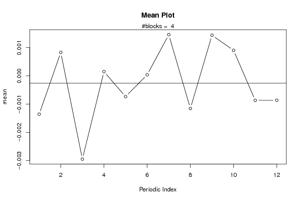
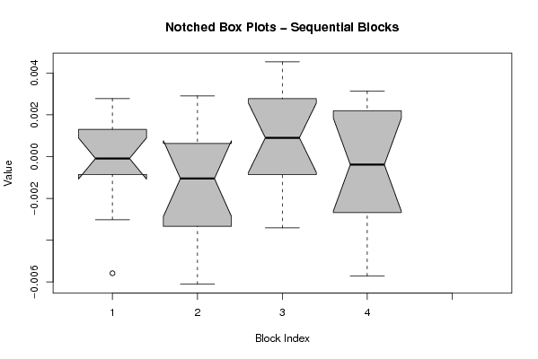
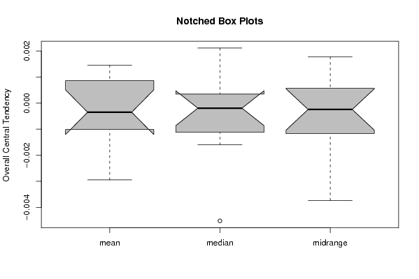
| Title produced by software | Mean Plot | ||||||||||||||||||||
| Date of computation | Tue, 08 Dec 2009 09:28:30 -0700 | ||||||||||||||||||||
| Cite this page as follows | Statistical Computations at FreeStatistics.org, Office for Research Development and Education, URL https://freestatistics.org/blog/index.php?v=date/2009/Dec/08/t1260289802cc9b2n3or9jpu5a.htm/, Retrieved Sat, 27 Apr 2024 19:37:34 +0000 | ||||||||||||||||||||
| Statistical Computations at FreeStatistics.org, Office for Research Development and Education, URL https://freestatistics.org/blog/index.php?pk=64728, Retrieved Sat, 27 Apr 2024 19:37:34 +0000 | |||||||||||||||||||||
| QR Codes: | |||||||||||||||||||||
|
| |||||||||||||||||||||
| Original text written by user: | |||||||||||||||||||||
| IsPrivate? | No (this computation is public) | ||||||||||||||||||||
| User-defined keywords | SDHW, DSHW | ||||||||||||||||||||
| Estimated Impact | 139 | ||||||||||||||||||||
Tree of Dependent Computations | |||||||||||||||||||||
| Family? (F = Feedback message, R = changed R code, M = changed R Module, P = changed Parameters, D = changed Data) | |||||||||||||||||||||
| - [Univariate Data Series] [data set] [2008-12-01 19:54:57] [b98453cac15ba1066b407e146608df68] - RMP [ARIMA Backward Selection] [] [2009-11-27 14:53:14] [b98453cac15ba1066b407e146608df68] - PD [ARIMA Backward Selection] [WS9 Berekening1 TVD] [2009-12-02 15:52:32] [42ad1186d39724f834063794eac7cea3] - [ARIMA Backward Selection] [TG 7] [2009-12-02 18:02:35] [a21bac9c8d3d56fdec8be4e719e2c7ed] - RMPD [Mean Plot] [DSHW-verbeteringWS91] [2009-12-08 16:28:30] [36295456a56d4c7dcc9b9537ce63463b] [Current] | |||||||||||||||||||||
| Feedback Forum | |||||||||||||||||||||
Post a new message | |||||||||||||||||||||
Dataset | |||||||||||||||||||||
| Dataseries X: | |||||||||||||||||||||
-0.000212923517308801 -0.000366405397205687 -0.00557947052088672 5.39349385913969e-05 0.00152371966762789 0.00175850683193595 3.77672323594971e-05 0.00278145948179106 -0.00301556173149557 0.00109580938363319 -0.000724132225897542 -0.000973482661448984 -0.00171178063930695 0.000125644167827909 -0.00610402063012358 -0.000405313640416258 7.26579064577097e-05 -0.00169069400551828 0.00113463103249704 -0.00502021989243185 0.00290671911265335 0.0026126296789493 -0.00247365301824070 -0.0041985012668281 0.00220019470292948 0.00403711355294332 0.00334851349840243 -0.00063160538606634 -0.000495111342862893 0.0019798998189597 0.00156938199908718 -0.00196786552076488 0.00453550691249892 0.000238202506318942 -0.00340957657161807 -0.00110204572510288 -0.00571315621593679 -0.000483401501108857 -0.00345934859091221 0.00157507010324105 -0.00404358222050192 -0.00189791760312953 0.00308855952516814 -0.000418917431675471 0.00131829063658993 -0.000343162709266577 0.00313721513408243 0.00281275625682837 | |||||||||||||||||||||
Tables (Output of Computation) | |||||||||||||||||||||
| |||||||||||||||||||||
Figures (Output of Computation) | |||||||||||||||||||||
Input Parameters & R Code | |||||||||||||||||||||
| Parameters (Session): | |||||||||||||||||||||
| par1 = 12 ; | |||||||||||||||||||||
| Parameters (R input): | |||||||||||||||||||||
| par1 = 12 ; | |||||||||||||||||||||
| R code (references can be found in the software module): | |||||||||||||||||||||
par1 <- as.numeric(par1) | |||||||||||||||||||||