Repository of Reproducible Computations

Free Statistics

of Irreproducible Research!

Author's title

Author

*The author of this computation has been verified*

R Software Module

rwasp_edauni.wasp

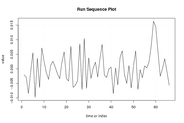
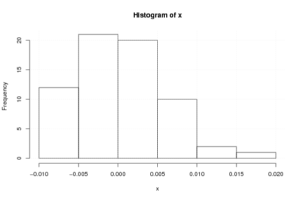
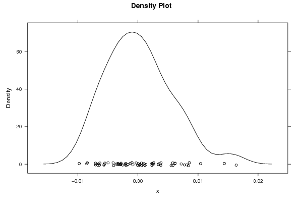
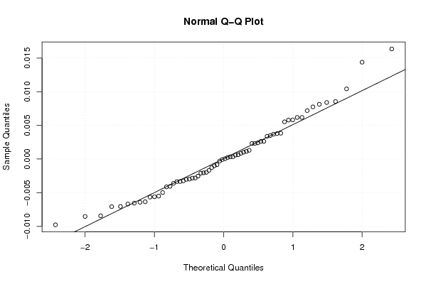
Title produced by software

Univariate Explorative Data Analysis

Date of computation

Tue, 08 Dec 2009 02:10:16 -0700

Cite this page as follows

Statistical Computations at FreeStatistics.org, Office for Research Development and Education, URL https://freestatistics.org/blog/index.php?v=date/2009/Dec/08/t1260263461blof8jt5gkuiopn.htm/, Retrieved Sun, 28 Apr 2024 05:02:35 +0000

Statistical Computations at FreeStatistics.org, Office for Research Development and Education, URL https://freestatistics.org/blog/index.php?pk=64682, Retrieved Sun, 28 Apr 2024 05:02:35 +0000

QR Codes:

Paste this QR Code to cite your computation.

Original text written by user:

IsPrivate?

No (this computation is public)

User-defined keywords

RWS9, uniEDA2

Estimated Impact

162

Family? (F = Feedback message, R = changed R code, M = changed R Module, P = changed Parameters, D = changed Data)

-     [Univariate Data Series] [data set] [2008-12-01 19:54:57] [b98453cac15ba1066b407e146608df68]
- RMP   [ARIMA Backward Selection] [] [2009-11-27 14:53:14] [b98453cac15ba1066b407e146608df68]
-    D    [ARIMA Backward Selection] [WS 9 Estimation o...] [2009-12-02 20:46:21] [101f710c1bf3d900563184d79f7da6e1]
-   PD      [ARIMA Backward Selection] [WS 9 Estimation o...] [2009-12-02 21:14:35] [101f710c1bf3d900563184d79f7da6e1]
- RMPD          [Univariate Explorative Data Analysis] [] [2009-12-08 09:10:16] [30f5b608e5a1bbbae86b1702c0071566] [Current]

Feedback Forum

Post a new message

Dataseries X:

Download CSV

Histogram

Boxplots

-0.00204571084483972 
-0.00283067359213242 
-0.0084361337759861 
-0.00100157883563286 
0.00552789133430058 
-0.0097773325684587 
0.0037008623592977 
-0.00642030822837614 
0.00719701196840899 
0.00262305115364016 
-0.00127110740029994 
-0.00361637523257659 
0.00129717707614950 
0.00261719199218297 
0.000582724800817553 
-0.00167915132702680 
-0.00335413275139399 
0.00232667127403374 
0.00582091392099778 
-0.00334066347103107 
-0.0041330370803219 
0.00774881947593112 
-0.00634148135279762 
-0.00566099578208234 
-0.00405877963621982 
0.0085509759075047 
-0.00707214396105319 
0.010425131510173 
-0.00668403745498932 
0.00379050813068932 
-0.00324993426129308 
0.000226742391370897 
0.00230434388712998 
-0.00281886460445299 
0.00337313318632658 
0.00840337336449575 
-0.00209978150552735 
-0.00297878965583557 
-8.0538712325838e-05 
0.000634354255519234 
-0.0085324150918054 
0.000335832194829364 
-0.00550713035158494 
0.00383522501954013 
0.00618077616849003 
-0.00197969322858899 
-0.00498017524803796 
0.00113774236948005 
-0.0065547872961444 
0.000839304818125273 
0.00617892965391168 
-0.00704587043257149 
-0.000296652134801466 
-0.003023626102382 
0.00101358450056993 
0.000322640390587606 
0.00241240601474065 
0.00813643317548373 
0.0163594234620832 
0.0143859819509878 
0.00578633446837098 
-0.00254190249003666 
4.37055206252088e-05 
0.00349291035208654 
-0.000839579699490873 
-0.00561011517767522

Summary of computational transaction
Raw Input	view raw input (R code)
Raw Output	view raw output of R engine
Computing time	3 seconds
R Server	'Gwilym Jenkins' @ 72.249.127.135

\begin{tabular}{lllllllll}
\hline
Summary of computational transaction \tabularnewline
Raw Input & view raw input (R code)  \tabularnewline
Raw Output & view raw output of R engine  \tabularnewline
Computing time & 3 seconds \tabularnewline
R Server & 'Gwilym Jenkins' @ 72.249.127.135 \tabularnewline
\hline
\end{tabular}
%Source: https://freestatistics.org/blog/index.php?pk=64682&T=0

[TABLE]
[ROW][C]Summary of computational transaction[/C][/ROW]
[ROW][C]Raw Input[/C][C]view raw input (R code) [/C][/ROW]
[ROW][C]Raw Output[/C][C]view raw output of R engine [/C][/ROW]
[ROW][C]Computing time[/C][C]3 seconds[/C][/ROW]
[ROW][C]R Server[/C][C]'Gwilym Jenkins' @ 72.249.127.135[/C][/ROW]
[/TABLE]
Source: https://freestatistics.org/blog/index.php?pk=64682&T=0

Globally Unique Identifier (entire table): ba.freestatistics.org/blog/index.php?pk=64682&T=0

As an alternative you can also use a QR Code:

The GUIDs for individual cells are displayed in the table below:

Summary of computational transaction
Raw Input	view raw input (R code)
Raw Output	view raw output of R engine
Computing time	3 seconds
R Server	'Gwilym Jenkins' @ 72.249.127.135

Descriptive Statistics
# observations	66
minimum	-0.0097773325684587
Q1	-0.00335076543130326
median	-1.84165958503146e-05
mean	0.000178009223653166
Q3	0.00346296606064655
maximum	0.0163594234620832

\begin{tabular}{lllllllll}
\hline
Descriptive Statistics \tabularnewline
# observations & 66 \tabularnewline
minimum & -0.0097773325684587 \tabularnewline
Q1 & -0.00335076543130326 \tabularnewline
median & -1.84165958503146e-05 \tabularnewline
mean & 0.000178009223653166 \tabularnewline
Q3 & 0.00346296606064655 \tabularnewline
maximum & 0.0163594234620832 \tabularnewline
\hline
\end{tabular}
%Source: https://freestatistics.org/blog/index.php?pk=64682&T=1

[TABLE]
[ROW][C]Descriptive Statistics[/C][/ROW]
[ROW][C]# observations[/C][C]66[/C][/ROW]
[ROW][C]minimum[/C][C]-0.0097773325684587[/C][/ROW]
[ROW][C]Q1[/C][C]-0.00335076543130326[/C][/ROW]
[ROW][C]median[/C][C]-1.84165958503146e-05[/C][/ROW]
[ROW][C]mean[/C][C]0.000178009223653166[/C][/ROW]
[ROW][C]Q3[/C][C]0.00346296606064655[/C][/ROW]
[ROW][C]maximum[/C][C]0.0163594234620832[/C][/ROW]
[/TABLE]
Source: https://freestatistics.org/blog/index.php?pk=64682&T=1

Globally Unique Identifier (entire table): ba.freestatistics.org/blog/index.php?pk=64682&T=1

As an alternative you can also use a QR Code:

The GUIDs for individual cells are displayed in the table below:

Descriptive Statistics
# observations	66
minimum	-0.0097773325684587
Q1	-0.00335076543130326
median	-1.84165958503146e-05
mean	0.000178009223653166
Q3	0.00346296606064655
maximum	0.0163594234620832

Figure 1

PNG link

Postscript link

PDF link

Figure 2

PNG link

Postscript link

PDF link

Figure 3

PNG link

Postscript link

PDF link

Figure 4

PNG link

Postscript link

PDF link

Figure 5

PNG link

Postscript link

PDF link

Figure 6

PNG link

Postscript link

PDF link

Figure 7

PNG link

Postscript link

PDF link

Parameters (Session):

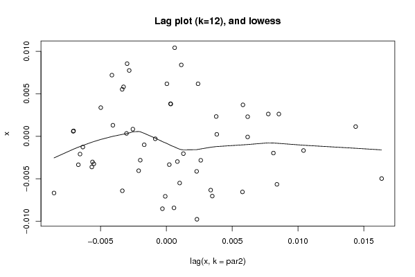
par1 = 0 ; par2 = 12 ;

Parameters (R input):

par1 = 0 ; par2 = 12 ;

R code (references can be found in the software module):

par1 <- as.numeric(par1)
par2 <- as.numeric(par2)
x <- as.ts(x)
library(lattice)
bitmap(file='pic1.png')
plot(x,type='l',main='Run Sequence Plot',xlab='time or index',ylab='value')
grid()
dev.off()
bitmap(file='pic2.png')
hist(x)
grid()
dev.off()
bitmap(file='pic3.png')
if (par1 > 0)
{
densityplot(~x,col='black',main=paste('Density Plot   bw = ',par1),bw=par1)
} else {
densityplot(~x,col='black',main='Density Plot')
}
dev.off()
bitmap(file='pic4.png')
qqnorm(x)
qqline(x)
grid()
dev.off()
if (par2 > 0)
{
bitmap(file='lagplot1.png')
dum <- cbind(lag(x,k=1),x)
dum
dum1 <- dum[2:length(x),]
dum1
z <- as.data.frame(dum1)
z
plot(z,main='Lag plot (k=1), lowess, and regression line')
lines(lowess(z))
abline(lm(z))
dev.off()
if (par2 > 1) {
bitmap(file='lagplotpar2.png')
dum <- cbind(lag(x,k=par2),x)
dum
dum1 <- dum[(par2+1):length(x),]
dum1
z <- as.data.frame(dum1)
z
mylagtitle <- 'Lag plot (k='
mylagtitle <- paste(mylagtitle,par2,sep='')
mylagtitle <- paste(mylagtitle,'), and lowess',sep='')
plot(z,main=mylagtitle)
lines(lowess(z))
dev.off()
}
bitmap(file='pic5.png')
acf(x,lag.max=par2,main='Autocorrelation Function')
grid()
dev.off()
}
summary(x)
load(file='createtable')
a<-table.start()
a<-table.row.start(a)
a<-table.element(a,'Descriptive Statistics',2,TRUE)
a<-table.row.end(a)
a<-table.row.start(a)
a<-table.element(a,'# observations',header=TRUE)
a<-table.element(a,length(x))
a<-table.row.end(a)
a<-table.row.start(a)
a<-table.element(a,'minimum',header=TRUE)
a<-table.element(a,min(x))
a<-table.row.end(a)
a<-table.row.start(a)
a<-table.element(a,'Q1',header=TRUE)
a<-table.element(a,quantile(x,0.25))
a<-table.row.end(a)
a<-table.row.start(a)
a<-table.element(a,'median',header=TRUE)
a<-table.element(a,median(x))
a<-table.row.end(a)
a<-table.row.start(a)
a<-table.element(a,'mean',header=TRUE)
a<-table.element(a,mean(x))
a<-table.row.end(a)
a<-table.row.start(a)
a<-table.element(a,'Q3',header=TRUE)
a<-table.element(a,quantile(x,0.75))
a<-table.row.end(a)
a<-table.row.start(a)
a<-table.element(a,'maximum',header=TRUE)
a<-table.element(a,max(x))
a<-table.row.end(a)
a<-table.end(a)
table.save(a,file='mytable.tab')

Free Statistics

Description of Statistical Computation

Tree of Dependent Computations

Dataset

Tables (Output of Computation)

Figures (Output of Computation)

Input Parameters & R Code