Free Statistics
of Irreproducible Research!
Description of Statistical Computation | |||||||||||||||||||||
|---|---|---|---|---|---|---|---|---|---|---|---|---|---|---|---|---|---|---|---|---|---|
| Author's title | |||||||||||||||||||||
| Author | *The author of this computation has been verified* | ||||||||||||||||||||
| R Software Module | rwasp_meanplot.wasp | ||||||||||||||||||||
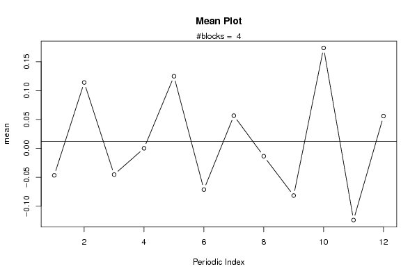
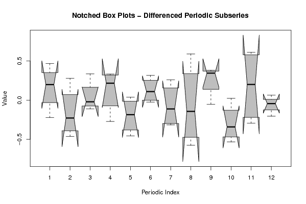
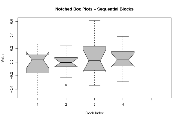
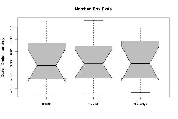
| Title produced by software | Mean Plot | ||||||||||||||||||||
| Date of computation | Mon, 07 Dec 2009 16:18:08 -0700 | ||||||||||||||||||||
| Cite this page as follows | Statistical Computations at FreeStatistics.org, Office for Research Development and Education, URL https://freestatistics.org/blog/index.php?v=date/2009/Dec/08/t1260227934rcciudm2apqflwn.htm/, Retrieved Sat, 27 Apr 2024 16:03:49 +0000 | ||||||||||||||||||||
| Statistical Computations at FreeStatistics.org, Office for Research Development and Education, URL https://freestatistics.org/blog/index.php?pk=64660, Retrieved Sat, 27 Apr 2024 16:03:49 +0000 | |||||||||||||||||||||
| QR Codes: | |||||||||||||||||||||
|
| |||||||||||||||||||||
| Original text written by user: | |||||||||||||||||||||
| IsPrivate? | No (this computation is public) | ||||||||||||||||||||
| User-defined keywords | |||||||||||||||||||||
| Estimated Impact | 176 | ||||||||||||||||||||
Tree of Dependent Computations | |||||||||||||||||||||
| Family? (F = Feedback message, R = changed R code, M = changed R Module, P = changed Parameters, D = changed Data) | |||||||||||||||||||||
| - [Univariate Data Series] [data set] [2008-12-01 19:54:57] [b98453cac15ba1066b407e146608df68] - RMP [ARIMA Backward Selection] [] [2009-11-27 14:53:14] [b98453cac15ba1066b407e146608df68] - PD [ARIMA Backward Selection] [] [2009-12-03 18:46:09] [90f6d58d515a4caed6fb4b8be4e11eaa] - RMPD [Mean Plot] [blog 3] [2009-12-07 20:35:48] [42ad1186d39724f834063794eac7cea3] - D [Mean Plot] [blog 12] [2009-12-07 23:18:08] [37de18e38c1490dd77c2b362ed87f3bb] [Current] | |||||||||||||||||||||
| Feedback Forum | |||||||||||||||||||||
Post a new message | |||||||||||||||||||||
Dataset | |||||||||||||||||||||
| Dataseries X: | |||||||||||||||||||||
0.0302547091228863 0.267612748598290 -0.05258221327681 -0.164815126360942 0.145251461046347 -0.159755000728184 0.0335569671830744 0.0880735117085241 -0.281966491596610 0.0474120142758863 -0.484987801933979 0.128597017186614 -0.0760862380652182 0.0847658982829797 -0.0514027132036804 -0.0566616141609282 0.069052111883504 0.00440676426158568 -0.0195453629146749 0.240643182454573 -0.33572474280097 0.0460275678865050 0.0696491220369025 -0.225076263667377 -0.161613617181671 0.306153117443247 -0.155979433289841 0.179413008162554 -0.0918257869952182 -0.0515872033510411 -0.0259692959341839 -0.341986993998746 0.248411293223152 0.610658133668028 0.207016437881814 0.0640914582469286 0.0207692245074071 -0.202335247943092 0.0784047280219788 0.0426875319465297 0.376752985339314 -0.0782742138517369 0.238382692897949 -0.0408923157917773 0.0426863373126538 -0.00863223279670068 -0.288046674979108 0.256083528841667 | |||||||||||||||||||||
Tables (Output of Computation) | |||||||||||||||||||||
| |||||||||||||||||||||
Figures (Output of Computation) | |||||||||||||||||||||
Input Parameters & R Code | |||||||||||||||||||||
| Parameters (Session): | |||||||||||||||||||||
| par1 = 12 ; | |||||||||||||||||||||
| Parameters (R input): | |||||||||||||||||||||
| par1 = 12 ; | |||||||||||||||||||||
| R code (references can be found in the software module): | |||||||||||||||||||||
par1 <- as.numeric(par1) | |||||||||||||||||||||