Free Statistics
of Irreproducible Research!
Description of Statistical Computation | |||||||||||||||||||||
|---|---|---|---|---|---|---|---|---|---|---|---|---|---|---|---|---|---|---|---|---|---|
| Author's title | |||||||||||||||||||||
| Author | *The author of this computation has been verified* | ||||||||||||||||||||
| R Software Module | rwasp_meanplot.wasp | ||||||||||||||||||||
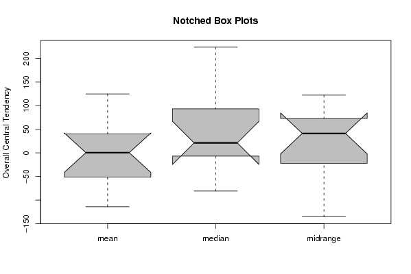
| Title produced by software | Mean Plot | ||||||||||||||||||||
| Date of computation | Mon, 07 Dec 2009 05:47:23 -0700 | ||||||||||||||||||||
| Cite this page as follows | Statistical Computations at FreeStatistics.org, Office for Research Development and Education, URL https://freestatistics.org/blog/index.php?v=date/2009/Dec/07/t12601902835woumjd1epmfa00.htm/, Retrieved Sun, 05 May 2024 10:18:42 +0000 | ||||||||||||||||||||
| Statistical Computations at FreeStatistics.org, Office for Research Development and Education, URL https://freestatistics.org/blog/index.php?pk=64562, Retrieved Sun, 05 May 2024 10:18:42 +0000 | |||||||||||||||||||||
| QR Codes: | |||||||||||||||||||||
|
| |||||||||||||||||||||
| Original text written by user: | |||||||||||||||||||||
| IsPrivate? | No (this computation is public) | ||||||||||||||||||||
| User-defined keywords | |||||||||||||||||||||
| Estimated Impact | 131 | ||||||||||||||||||||
Tree of Dependent Computations | |||||||||||||||||||||
| Family? (F = Feedback message, R = changed R code, M = changed R Module, P = changed Parameters, D = changed Data) | |||||||||||||||||||||
| - [Univariate Data Series] [data set] [2008-12-01 19:54:57] [b98453cac15ba1066b407e146608df68] - RMP [ARIMA Backward Selection] [] [2009-11-27 14:53:14] [b98453cac15ba1066b407e146608df68] - R PD [ARIMA Backward Selection] [] [2009-12-04 08:49:16] [1e83ffa964db6f7ea6ccc4e7b5acbbff] - RMPD [Mean Plot] [verbetering workshop] [2009-12-07 12:47:23] [b32ceebc68d054278e6bda97f3d57f91] [Current] | |||||||||||||||||||||
| Feedback Forum | |||||||||||||||||||||
Post a new message | |||||||||||||||||||||
Dataset | |||||||||||||||||||||
| Dataseries X: | |||||||||||||||||||||
2.75675840647712 86.0377999064762 42.9984522539679 33.5054449351983 62.9132382279737 -16.4128806120557 -6.52270297513587 -82.2241535106955 46.5759071081666 51.7913037642593 89.9736608618232 -13.7769558605610 -0.547498629244274 43.7484112333814 107.260977054051 133.441764601343 84.4357033956076 37.8119274071482 -87.1935455457301 -118.771969577577 -226.993428652981 199.325523642462 144.404698877001 112.069029838591 111.504792874925 -18.3387880730807 51.9033275846095 92.9654085924249 4.11307164252776 -180.731575979433 242.202806283966 29.3705651270102 -74.0779181790358 -86.7691638153374 -366.352653743473 208.264095886472 125.258399413132 -292.828740889365 82.153399145297 -304.275237560671 19.7695007775624 -15.2039496812031 252.735165584425 -80.8995541445702 -271.506819998227 -428.856283523052 155.237771456622 -26.7479776990567 -642.951943053832 22.6846703389315 -83.8099608577902 243.516820340160 -67.8138203680369 -83.4728588077735 224.023836737227 154.123353862388 -44.3201964833738 6.8163473353593 172.177056551561 93.6702465237527 | |||||||||||||||||||||
Tables (Output of Computation) | |||||||||||||||||||||
| |||||||||||||||||||||
Figures (Output of Computation) | |||||||||||||||||||||
Input Parameters & R Code | |||||||||||||||||||||
| Parameters (Session): | |||||||||||||||||||||
| par1 = 12 ; | |||||||||||||||||||||
| Parameters (R input): | |||||||||||||||||||||
| par1 = 12 ; | |||||||||||||||||||||
| R code (references can be found in the software module): | |||||||||||||||||||||
par1 <- as.numeric(par1) | |||||||||||||||||||||