Free Statistics
of Irreproducible Research!
Description of Statistical Computation | |||||||||||||||||||||
|---|---|---|---|---|---|---|---|---|---|---|---|---|---|---|---|---|---|---|---|---|---|
| Author's title | |||||||||||||||||||||
| Author | *The author of this computation has been verified* | ||||||||||||||||||||
| R Software Module | rwasp_meanplot.wasp | ||||||||||||||||||||
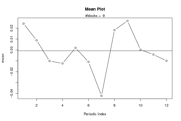
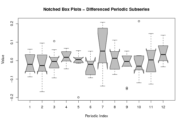
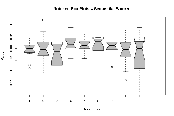
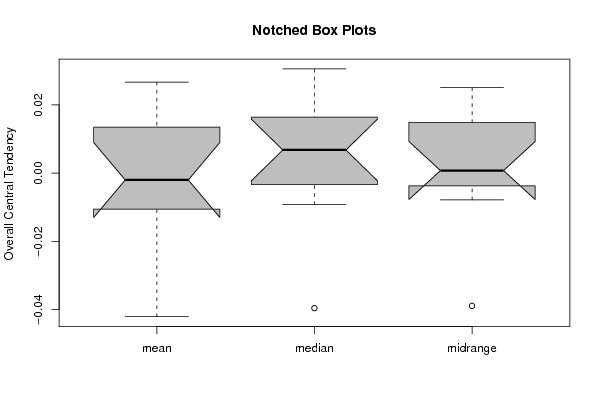
| Title produced by software | Mean Plot | ||||||||||||||||||||
| Date of computation | Thu, 03 Dec 2009 10:44:27 -0700 | ||||||||||||||||||||
| Cite this page as follows | Statistical Computations at FreeStatistics.org, Office for Research Development and Education, URL https://freestatistics.org/blog/index.php?v=date/2009/Dec/03/t1259862311m50jmj3gr4ru3k3.htm/, Retrieved Wed, 09 Jul 2025 16:16:00 +0000 | ||||||||||||||||||||
| Statistical Computations at FreeStatistics.org, Office for Research Development and Education, URL https://freestatistics.org/blog/index.php?pk=62976, Retrieved Wed, 09 Jul 2025 16:16:00 +0000 | |||||||||||||||||||||
| QR Codes: | |||||||||||||||||||||
|
| |||||||||||||||||||||
| Original text written by user: | |||||||||||||||||||||
| IsPrivate? | No (this computation is public) | ||||||||||||||||||||
| User-defined keywords | |||||||||||||||||||||
| Estimated Impact | 228 | ||||||||||||||||||||
Tree of Dependent Computations | |||||||||||||||||||||
| Family? (F = Feedback message, R = changed R code, M = changed R Module, P = changed Parameters, D = changed Data) | |||||||||||||||||||||
| - [Univariate Data Series] [data set] [2008-12-01 19:54:57] [b98453cac15ba1066b407e146608df68] - RMP [ARIMA Backward Selection] [] [2009-11-27 14:53:14] [b98453cac15ba1066b407e146608df68] - PD [ARIMA Backward Selection] [workshop 9 bereke...] [2009-12-03 17:01:00] [eaf42bcf5162b5692bb3c7f9d4636222] - RM D [Harrell-Davis Quantiles] [workshop 9 bereke...] [2009-12-03 17:33:57] [eaf42bcf5162b5692bb3c7f9d4636222] - RM [Mean Plot] [workshop 9 bereke...] [2009-12-03 17:44:27] [78d370e6d5f4594e9982a5085e7604c6] [Current] | |||||||||||||||||||||
| Feedback Forum | |||||||||||||||||||||
Post a new message | |||||||||||||||||||||
Dataset | |||||||||||||||||||||
| Dataseries X: | |||||||||||||||||||||
0.00542916130943278 0.0445893441667106 -0.0137888879399847 0.0453152005372048 0.00473315051318341 -0.00629302867546508 -0.070117568265751 -0.0217843333183126 -0.0095666262457008 0.0165637840451361 0.00824993070407797 -0.0831327333629231 0.0144161451837631 0.034621459194465 0.0184381942383567 -0.074932085622151 -0.0264502766059977 -0.0112128979582415 -0.10436727046515 0.0715680268198404 0.121060489346963 -0.0324214631834054 -0.00529431524629609 -0.00146846269678377 -0.00570151995165197 -0.025987421858386 -0.0685516945712228 -0.0733842752561877 -0.0163445778492365 -0.0110134858421602 -0.087660645529663 0.109058909700739 0.0339807510912559 0.00300957055239715 -0.117182246964976 0.0294137488267335 0.0893484543689374 0.0298847434899963 0.0611729025233987 0.00324519869485862 0.0212178770497218 0.00660658211635031 0.00372487320385017 -0.00838101340628686 0.0170033508018199 0.0621313219493351 0.0197401442742924 -0.0417164562197347 0.0228259755720078 -0.042255817474836 0.0309137428469852 -0.00918278678351927 0.0146293075798733 0.0297847213520409 0.00986110949240185 0.0614197587407885 0.0126952510044700 0.00800151002534761 0.0341797308392325 -0.0180464496214532 -0.0153479524622885 0.0463170445239729 0.0195281991212937 0.0371269245007414 -0.00744692508954433 0.0462493884790173 -0.0395877264208058 0.0382572916842234 0.0374023801364467 0.039717646637445 -0.0103197596326754 0.00344718875977555 0.00885007204463633 -0.0791417702355047 0.0158234735164099 0.016538541536172 0.0144056817515094 0.00282613662406027 0.0534415346690993 -0.0114429989198319 0.0380793061367662 0.0110221503256857 -0.0190504147856999 0.0414994449048327 0.00816603652061595 0.041019836581154 -0.0171632971999998 -0.0239258971120320 -0.0219604522663097 0.00948947211086537 0.039949080719774 -0.0982011343440696 0.0127754891139968 -0.134456574642575 0.0790854375582093 -0.0486237536443106 0.0893991774345677 0.0305540121228036 -0.137690614650960 -0.0322141353773482 0.03442439486507 -0.164911125871352 -0.183934800698021 0.0234325246699871 -0.0233244578414444 0.0283600031799320 -0.0273434825220074 0.0285743363772815 | |||||||||||||||||||||
Tables (Output of Computation) | |||||||||||||||||||||
| |||||||||||||||||||||
Figures (Output of Computation) | |||||||||||||||||||||
Input Parameters & R Code | |||||||||||||||||||||
| Parameters (Session): | |||||||||||||||||||||
| par1 = FALSE ; par2 = 0.2 ; par3 = 1 ; par4 = 0 ; par5 = 12 ; par6 = 2 ; par7 = 0 ; par8 = 0 ; par9 = 0 ; | |||||||||||||||||||||
| Parameters (R input): | |||||||||||||||||||||
| par1 = 12 ; | |||||||||||||||||||||
| R code (references can be found in the software module): | |||||||||||||||||||||
par1 <- as.numeric(par1) | |||||||||||||||||||||