Repository of Reproducible Computations

Free Statistics

of Irreproducible Research!

Author's title

Author

*The author of this computation has been verified*

R Software Module

rwasp_autocorrelation.wasp

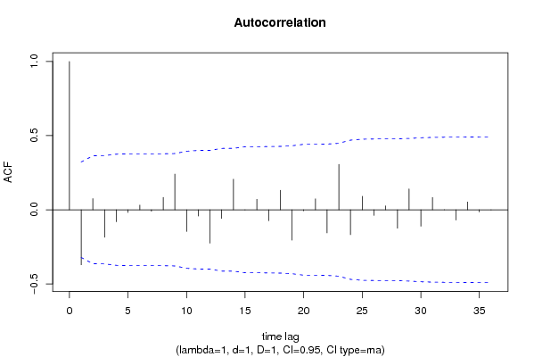
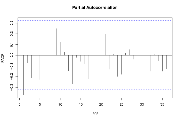
Title produced by software

(Partial) Autocorrelation Function

Date of computation

Thu, 03 Dec 2009 08:46:01 -0700

Cite this page as follows

Statistical Computations at FreeStatistics.org, Office for Research Development and Education, URL https://freestatistics.org/blog/index.php?v=date/2009/Dec/03/t12598552619utkoct8zhoknnj.htm/, Retrieved Fri, 19 Apr 2024 12:59:22 +0000

Statistical Computations at FreeStatistics.org, Office for Research Development and Education, URL https://freestatistics.org/blog/index.php?pk=62852, Retrieved Fri, 19 Apr 2024 12:59:22 +0000

QR Codes:

Paste this QR Code to cite your computation.

Original text written by user:

IsPrivate?

No (this computation is public)

User-defined keywords

Estimated Impact

142

Family? (F = Feedback message, R = changed R code, M = changed R Module, P = changed Parameters, D = changed Data)

-     [Univariate Explorative Data Analysis] [Run Sequence gebo...] [2008-12-12 13:32:37] [76963dc1903f0f612b6153510a3818cf]
- R  D  [Univariate Explorative Data Analysis] [Run Sequence gebo...] [2008-12-17 12:14:40] [76963dc1903f0f612b6153510a3818cf]
-         [Univariate Explorative Data Analysis] [Run Sequence Plot...] [2008-12-22 18:19:51] [1ce0d16c8f4225c977b42c8fa93bc163]
- RMP       [(Partial) Autocorrelation Function] [Identifying Integ...] [2009-11-22 12:19:56] [b98453cac15ba1066b407e146608df68]
-    D        [(Partial) Autocorrelation Function] [] [2009-11-25 12:07:39] [d811f621c525a990f9b60f1ae1e2e8fd]
-   P             [(Partial) Autocorrelation Function] [ACF D=1, d=1] [2009-12-03 15:46:01] [d1818fb1d9a1b0f34f8553ada228d3d5] [Current]

Feedback Forum

Post a new message

Dataseries X:

Download CSV

Histogram

Boxplots

Summary of computational transaction
Raw Input	view raw input (R code)
Raw Output	view raw output of R engine
Computing time	1 seconds
R Server	'Gwilym Jenkins' @ 72.249.127.135

\begin{tabular}{lllllllll}
\hline
Summary of computational transaction \tabularnewline
Raw Input & view raw input (R code)  \tabularnewline
Raw Output & view raw output of R engine  \tabularnewline
Computing time & 1 seconds \tabularnewline
R Server & 'Gwilym Jenkins' @ 72.249.127.135 \tabularnewline
\hline
\end{tabular}
%Source: https://freestatistics.org/blog/index.php?pk=62852&T=0

[TABLE]
[ROW][C]Summary of computational transaction[/C][/ROW]
[ROW][C]Raw Input[/C][C]view raw input (R code) [/C][/ROW]
[ROW][C]Raw Output[/C][C]view raw output of R engine [/C][/ROW]
[ROW][C]Computing time[/C][C]1 seconds[/C][/ROW]
[ROW][C]R Server[/C][C]'Gwilym Jenkins' @ 72.249.127.135[/C][/ROW]
[/TABLE]
Source: https://freestatistics.org/blog/index.php?pk=62852&T=0

Globally Unique Identifier (entire table): ba.freestatistics.org/blog/index.php?pk=62852&T=0

As an alternative you can also use a QR Code:

The GUIDs for individual cells are displayed in the table below:

Summary of computational transaction
Raw Input	view raw input (R code)
Raw Output	view raw output of R engine
Computing time	1 seconds
R Server	'Gwilym Jenkins' @ 72.249.127.135

Autocorrelation Function
Time lag k	ACF(k)	T-STAT	P-value
1	-0.371247	-2.2582	0.014959
2	0.074797	0.455	0.325894
3	-0.185341	-1.1274	0.133419
4	-0.0811	-0.4933	0.312353
5	-0.018618	-0.1132	0.455223
6	0.0316	0.1922	0.424311
7	-0.010277	-0.0625	0.475245
8	0.083603	0.5085	0.307048
9	0.240426	1.4625	0.076029
10	-0.146041	-0.8883	0.19005
11	-0.042748	-0.26	0.398143
12	-0.225041	-1.3689	0.089646
13	-0.058094	-0.3534	0.362907
14	0.205694	1.2512	0.10936
15	-0.000943	-0.0057	0.497727
16	0.070477	0.4287	0.335315
17	-0.073805	-0.4489	0.328048
18	0.131239	0.7983	0.214897
19	-0.205406	-1.2494	0.109676
20	-0.007347	-0.0447	0.482298
21	0.073211	0.4453	0.329339
22	-0.156215	-0.9502	0.174083
23	0.306085	1.8618	0.035292
24	-0.167981	-1.0218	0.156757
25	0.09042	0.55	0.29281
26	-0.037919	-0.2307	0.409427
27	0.025996	0.1581	0.437607
28	-0.124629	-0.7581	0.2266
29	0.140264	0.8532	0.199522
30	-0.110634	-0.673	0.252578
31	0.082737	0.5033	0.308879
32	-0.000198	-0.0012	0.499522
33	-0.069761	-0.4243	0.336889
34	0.052611	0.32	0.375376
35	-0.014369	-0.0874	0.465412
36	-0.001447	-0.0088	0.496513

\begin{tabular}{lllllllll}
\hline
Autocorrelation Function \tabularnewline
Time lag k & ACF(k) & T-STAT & P-value \tabularnewline
1 & -0.371247 & -2.2582 & 0.014959 \tabularnewline
2 & 0.074797 & 0.455 & 0.325894 \tabularnewline
3 & -0.185341 & -1.1274 & 0.133419 \tabularnewline
4 & -0.0811 & -0.4933 & 0.312353 \tabularnewline
5 & -0.018618 & -0.1132 & 0.455223 \tabularnewline
6 & 0.0316 & 0.1922 & 0.424311 \tabularnewline
7 & -0.010277 & -0.0625 & 0.475245 \tabularnewline
8 & 0.083603 & 0.5085 & 0.307048 \tabularnewline
9 & 0.240426 & 1.4625 & 0.076029 \tabularnewline
10 & -0.146041 & -0.8883 & 0.19005 \tabularnewline
11 & -0.042748 & -0.26 & 0.398143 \tabularnewline
12 & -0.225041 & -1.3689 & 0.089646 \tabularnewline
13 & -0.058094 & -0.3534 & 0.362907 \tabularnewline
14 & 0.205694 & 1.2512 & 0.10936 \tabularnewline
15 & -0.000943 & -0.0057 & 0.497727 \tabularnewline
16 & 0.070477 & 0.4287 & 0.335315 \tabularnewline
17 & -0.073805 & -0.4489 & 0.328048 \tabularnewline
18 & 0.131239 & 0.7983 & 0.214897 \tabularnewline
19 & -0.205406 & -1.2494 & 0.109676 \tabularnewline
20 & -0.007347 & -0.0447 & 0.482298 \tabularnewline
21 & 0.073211 & 0.4453 & 0.329339 \tabularnewline
22 & -0.156215 & -0.9502 & 0.174083 \tabularnewline
23 & 0.306085 & 1.8618 & 0.035292 \tabularnewline
24 & -0.167981 & -1.0218 & 0.156757 \tabularnewline
25 & 0.09042 & 0.55 & 0.29281 \tabularnewline
26 & -0.037919 & -0.2307 & 0.409427 \tabularnewline
27 & 0.025996 & 0.1581 & 0.437607 \tabularnewline
28 & -0.124629 & -0.7581 & 0.2266 \tabularnewline
29 & 0.140264 & 0.8532 & 0.199522 \tabularnewline
30 & -0.110634 & -0.673 & 0.252578 \tabularnewline
31 & 0.082737 & 0.5033 & 0.308879 \tabularnewline
32 & -0.000198 & -0.0012 & 0.499522 \tabularnewline
33 & -0.069761 & -0.4243 & 0.336889 \tabularnewline
34 & 0.052611 & 0.32 & 0.375376 \tabularnewline
35 & -0.014369 & -0.0874 & 0.465412 \tabularnewline
36 & -0.001447 & -0.0088 & 0.496513 \tabularnewline
\hline
\end{tabular}
%Source: https://freestatistics.org/blog/index.php?pk=62852&T=1

[TABLE]
[ROW][C]Autocorrelation Function[/C][/ROW]
[ROW][C]Time lag k[/C][C]ACF(k)[/C][C]T-STAT[/C][C]P-value[/C][/ROW]
[ROW][C]1[/C][C]-0.371247[/C][C]-2.2582[/C][C]0.014959[/C][/ROW]
[ROW][C]2[/C][C]0.074797[/C][C]0.455[/C][C]0.325894[/C][/ROW]
[ROW][C]3[/C][C]-0.185341[/C][C]-1.1274[/C][C]0.133419[/C][/ROW]
[ROW][C]4[/C][C]-0.0811[/C][C]-0.4933[/C][C]0.312353[/C][/ROW]
[ROW][C]5[/C][C]-0.018618[/C][C]-0.1132[/C][C]0.455223[/C][/ROW]
[ROW][C]6[/C][C]0.0316[/C][C]0.1922[/C][C]0.424311[/C][/ROW]
[ROW][C]7[/C][C]-0.010277[/C][C]-0.0625[/C][C]0.475245[/C][/ROW]
[ROW][C]8[/C][C]0.083603[/C][C]0.5085[/C][C]0.307048[/C][/ROW]
[ROW][C]9[/C][C]0.240426[/C][C]1.4625[/C][C]0.076029[/C][/ROW]
[ROW][C]10[/C][C]-0.146041[/C][C]-0.8883[/C][C]0.19005[/C][/ROW]
[ROW][C]11[/C][C]-0.042748[/C][C]-0.26[/C][C]0.398143[/C][/ROW]
[ROW][C]12[/C][C]-0.225041[/C][C]-1.3689[/C][C]0.089646[/C][/ROW]
[ROW][C]13[/C][C]-0.058094[/C][C]-0.3534[/C][C]0.362907[/C][/ROW]
[ROW][C]14[/C][C]0.205694[/C][C]1.2512[/C][C]0.10936[/C][/ROW]
[ROW][C]15[/C][C]-0.000943[/C][C]-0.0057[/C][C]0.497727[/C][/ROW]
[ROW][C]16[/C][C]0.070477[/C][C]0.4287[/C][C]0.335315[/C][/ROW]
[ROW][C]17[/C][C]-0.073805[/C][C]-0.4489[/C][C]0.328048[/C][/ROW]
[ROW][C]18[/C][C]0.131239[/C][C]0.7983[/C][C]0.214897[/C][/ROW]
[ROW][C]19[/C][C]-0.205406[/C][C]-1.2494[/C][C]0.109676[/C][/ROW]
[ROW][C]20[/C][C]-0.007347[/C][C]-0.0447[/C][C]0.482298[/C][/ROW]
[ROW][C]21[/C][C]0.073211[/C][C]0.4453[/C][C]0.329339[/C][/ROW]
[ROW][C]22[/C][C]-0.156215[/C][C]-0.9502[/C][C]0.174083[/C][/ROW]
[ROW][C]23[/C][C]0.306085[/C][C]1.8618[/C][C]0.035292[/C][/ROW]
[ROW][C]24[/C][C]-0.167981[/C][C]-1.0218[/C][C]0.156757[/C][/ROW]
[ROW][C]25[/C][C]0.09042[/C][C]0.55[/C][C]0.29281[/C][/ROW]
[ROW][C]26[/C][C]-0.037919[/C][C]-0.2307[/C][C]0.409427[/C][/ROW]
[ROW][C]27[/C][C]0.025996[/C][C]0.1581[/C][C]0.437607[/C][/ROW]
[ROW][C]28[/C][C]-0.124629[/C][C]-0.7581[/C][C]0.2266[/C][/ROW]
[ROW][C]29[/C][C]0.140264[/C][C]0.8532[/C][C]0.199522[/C][/ROW]
[ROW][C]30[/C][C]-0.110634[/C][C]-0.673[/C][C]0.252578[/C][/ROW]
[ROW][C]31[/C][C]0.082737[/C][C]0.5033[/C][C]0.308879[/C][/ROW]
[ROW][C]32[/C][C]-0.000198[/C][C]-0.0012[/C][C]0.499522[/C][/ROW]
[ROW][C]33[/C][C]-0.069761[/C][C]-0.4243[/C][C]0.336889[/C][/ROW]
[ROW][C]34[/C][C]0.052611[/C][C]0.32[/C][C]0.375376[/C][/ROW]
[ROW][C]35[/C][C]-0.014369[/C][C]-0.0874[/C][C]0.465412[/C][/ROW]
[ROW][C]36[/C][C]-0.001447[/C][C]-0.0088[/C][C]0.496513[/C][/ROW]
[/TABLE]
Source: https://freestatistics.org/blog/index.php?pk=62852&T=1

Globally Unique Identifier (entire table): ba.freestatistics.org/blog/index.php?pk=62852&T=1

As an alternative you can also use a QR Code:

The GUIDs for individual cells are displayed in the table below:

Autocorrelation Function
Time lag k	ACF(k)	T-STAT	P-value
1	-0.371247	-2.2582	0.014959
2	0.074797	0.455	0.325894
3	-0.185341	-1.1274	0.133419
4	-0.0811	-0.4933	0.312353
5	-0.018618	-0.1132	0.455223
6	0.0316	0.1922	0.424311
7	-0.010277	-0.0625	0.475245
8	0.083603	0.5085	0.307048
9	0.240426	1.4625	0.076029
10	-0.146041	-0.8883	0.19005
11	-0.042748	-0.26	0.398143
12	-0.225041	-1.3689	0.089646
13	-0.058094	-0.3534	0.362907
14	0.205694	1.2512	0.10936
15	-0.000943	-0.0057	0.497727
16	0.070477	0.4287	0.335315
17	-0.073805	-0.4489	0.328048
18	0.131239	0.7983	0.214897
19	-0.205406	-1.2494	0.109676
20	-0.007347	-0.0447	0.482298
21	0.073211	0.4453	0.329339
22	-0.156215	-0.9502	0.174083
23	0.306085	1.8618	0.035292
24	-0.167981	-1.0218	0.156757
25	0.09042	0.55	0.29281
26	-0.037919	-0.2307	0.409427
27	0.025996	0.1581	0.437607
28	-0.124629	-0.7581	0.2266
29	0.140264	0.8532	0.199522
30	-0.110634	-0.673	0.252578
31	0.082737	0.5033	0.308879
32	-0.000198	-0.0012	0.499522
33	-0.069761	-0.4243	0.336889
34	0.052611	0.32	0.375376
35	-0.014369	-0.0874	0.465412
36	-0.001447	-0.0088	0.496513

Partial Autocorrelation Function
Time lag k	PACF(k)	T-STAT	P-value
1	-0.371247	-2.2582	0.014959
2	-0.073103	-0.4447	0.329575
3	-0.213023	-1.2958	0.10154
4	-0.274955	-1.6725	0.051433
5	-0.227149	-1.3817	0.087676
6	-0.174869	-1.0637	0.147182
7	-0.222364	-1.3526	0.092198
8	-0.144903	-0.8814	0.191892
9	0.248599	1.5122	0.069493
10	0.121123	0.7368	0.232956
11	0.030224	0.1838	0.42757
12	-0.147543	-0.8975	0.187636
13	-0.270543	-1.6456	0.054153
14	-0.020677	-0.1258	0.450295
15	-0.058311	-0.3547	0.362416
16	-0.079747	-0.4851	0.315239
17	-0.221183	-1.3454	0.093342
18	-0.033867	-0.206	0.418958
19	-0.168699	-1.0262	0.15574
20	-0.216864	-1.3191	0.097616
21	0.195177	1.1872	0.121355
22	-0.131459	-0.7996	0.214514
23	0.006595	0.0401	0.484108
24	-0.198549	-1.2077	0.117408
25	-0.179043	-1.0891	0.141581
26	0.01938	0.1179	0.453399
27	0.053459	0.3252	0.373439
28	-0.037515	-0.2282	0.410376
29	0.016353	0.0995	0.460651
30	-0.08305	-0.5052	0.308217
31	-0.003563	-0.0217	0.491414
32	-0.148624	-0.904	0.18591
33	0.008941	0.0544	0.478461
34	-0.053634	-0.3262	0.37304
35	-0.149629	-0.9102	0.184316
36	-0.129448	-0.7874	0.218031

\begin{tabular}{lllllllll}
\hline
Partial Autocorrelation Function \tabularnewline
Time lag k & PACF(k) & T-STAT & P-value \tabularnewline
1 & -0.371247 & -2.2582 & 0.014959 \tabularnewline
2 & -0.073103 & -0.4447 & 0.329575 \tabularnewline
3 & -0.213023 & -1.2958 & 0.10154 \tabularnewline
4 & -0.274955 & -1.6725 & 0.051433 \tabularnewline
5 & -0.227149 & -1.3817 & 0.087676 \tabularnewline
6 & -0.174869 & -1.0637 & 0.147182 \tabularnewline
7 & -0.222364 & -1.3526 & 0.092198 \tabularnewline
8 & -0.144903 & -0.8814 & 0.191892 \tabularnewline
9 & 0.248599 & 1.5122 & 0.069493 \tabularnewline
10 & 0.121123 & 0.7368 & 0.232956 \tabularnewline
11 & 0.030224 & 0.1838 & 0.42757 \tabularnewline
12 & -0.147543 & -0.8975 & 0.187636 \tabularnewline
13 & -0.270543 & -1.6456 & 0.054153 \tabularnewline
14 & -0.020677 & -0.1258 & 0.450295 \tabularnewline
15 & -0.058311 & -0.3547 & 0.362416 \tabularnewline
16 & -0.079747 & -0.4851 & 0.315239 \tabularnewline
17 & -0.221183 & -1.3454 & 0.093342 \tabularnewline
18 & -0.033867 & -0.206 & 0.418958 \tabularnewline
19 & -0.168699 & -1.0262 & 0.15574 \tabularnewline
20 & -0.216864 & -1.3191 & 0.097616 \tabularnewline
21 & 0.195177 & 1.1872 & 0.121355 \tabularnewline
22 & -0.131459 & -0.7996 & 0.214514 \tabularnewline
23 & 0.006595 & 0.0401 & 0.484108 \tabularnewline
24 & -0.198549 & -1.2077 & 0.117408 \tabularnewline
25 & -0.179043 & -1.0891 & 0.141581 \tabularnewline
26 & 0.01938 & 0.1179 & 0.453399 \tabularnewline
27 & 0.053459 & 0.3252 & 0.373439 \tabularnewline
28 & -0.037515 & -0.2282 & 0.410376 \tabularnewline
29 & 0.016353 & 0.0995 & 0.460651 \tabularnewline
30 & -0.08305 & -0.5052 & 0.308217 \tabularnewline
31 & -0.003563 & -0.0217 & 0.491414 \tabularnewline
32 & -0.148624 & -0.904 & 0.18591 \tabularnewline
33 & 0.008941 & 0.0544 & 0.478461 \tabularnewline
34 & -0.053634 & -0.3262 & 0.37304 \tabularnewline
35 & -0.149629 & -0.9102 & 0.184316 \tabularnewline
36 & -0.129448 & -0.7874 & 0.218031 \tabularnewline
\hline
\end{tabular}
%Source: https://freestatistics.org/blog/index.php?pk=62852&T=2

[TABLE]
[ROW][C]Partial Autocorrelation Function[/C][/ROW]
[ROW][C]Time lag k[/C][C]PACF(k)[/C][C]T-STAT[/C][C]P-value[/C][/ROW]
[ROW][C]1[/C][C]-0.371247[/C][C]-2.2582[/C][C]0.014959[/C][/ROW]
[ROW][C]2[/C][C]-0.073103[/C][C]-0.4447[/C][C]0.329575[/C][/ROW]
[ROW][C]3[/C][C]-0.213023[/C][C]-1.2958[/C][C]0.10154[/C][/ROW]
[ROW][C]4[/C][C]-0.274955[/C][C]-1.6725[/C][C]0.051433[/C][/ROW]
[ROW][C]5[/C][C]-0.227149[/C][C]-1.3817[/C][C]0.087676[/C][/ROW]
[ROW][C]6[/C][C]-0.174869[/C][C]-1.0637[/C][C]0.147182[/C][/ROW]
[ROW][C]7[/C][C]-0.222364[/C][C]-1.3526[/C][C]0.092198[/C][/ROW]
[ROW][C]8[/C][C]-0.144903[/C][C]-0.8814[/C][C]0.191892[/C][/ROW]
[ROW][C]9[/C][C]0.248599[/C][C]1.5122[/C][C]0.069493[/C][/ROW]
[ROW][C]10[/C][C]0.121123[/C][C]0.7368[/C][C]0.232956[/C][/ROW]
[ROW][C]11[/C][C]0.030224[/C][C]0.1838[/C][C]0.42757[/C][/ROW]
[ROW][C]12[/C][C]-0.147543[/C][C]-0.8975[/C][C]0.187636[/C][/ROW]
[ROW][C]13[/C][C]-0.270543[/C][C]-1.6456[/C][C]0.054153[/C][/ROW]
[ROW][C]14[/C][C]-0.020677[/C][C]-0.1258[/C][C]0.450295[/C][/ROW]
[ROW][C]15[/C][C]-0.058311[/C][C]-0.3547[/C][C]0.362416[/C][/ROW]
[ROW][C]16[/C][C]-0.079747[/C][C]-0.4851[/C][C]0.315239[/C][/ROW]
[ROW][C]17[/C][C]-0.221183[/C][C]-1.3454[/C][C]0.093342[/C][/ROW]
[ROW][C]18[/C][C]-0.033867[/C][C]-0.206[/C][C]0.418958[/C][/ROW]
[ROW][C]19[/C][C]-0.168699[/C][C]-1.0262[/C][C]0.15574[/C][/ROW]
[ROW][C]20[/C][C]-0.216864[/C][C]-1.3191[/C][C]0.097616[/C][/ROW]
[ROW][C]21[/C][C]0.195177[/C][C]1.1872[/C][C]0.121355[/C][/ROW]
[ROW][C]22[/C][C]-0.131459[/C][C]-0.7996[/C][C]0.214514[/C][/ROW]
[ROW][C]23[/C][C]0.006595[/C][C]0.0401[/C][C]0.484108[/C][/ROW]
[ROW][C]24[/C][C]-0.198549[/C][C]-1.2077[/C][C]0.117408[/C][/ROW]
[ROW][C]25[/C][C]-0.179043[/C][C]-1.0891[/C][C]0.141581[/C][/ROW]
[ROW][C]26[/C][C]0.01938[/C][C]0.1179[/C][C]0.453399[/C][/ROW]
[ROW][C]27[/C][C]0.053459[/C][C]0.3252[/C][C]0.373439[/C][/ROW]
[ROW][C]28[/C][C]-0.037515[/C][C]-0.2282[/C][C]0.410376[/C][/ROW]
[ROW][C]29[/C][C]0.016353[/C][C]0.0995[/C][C]0.460651[/C][/ROW]
[ROW][C]30[/C][C]-0.08305[/C][C]-0.5052[/C][C]0.308217[/C][/ROW]
[ROW][C]31[/C][C]-0.003563[/C][C]-0.0217[/C][C]0.491414[/C][/ROW]
[ROW][C]32[/C][C]-0.148624[/C][C]-0.904[/C][C]0.18591[/C][/ROW]
[ROW][C]33[/C][C]0.008941[/C][C]0.0544[/C][C]0.478461[/C][/ROW]
[ROW][C]34[/C][C]-0.053634[/C][C]-0.3262[/C][C]0.37304[/C][/ROW]
[ROW][C]35[/C][C]-0.149629[/C][C]-0.9102[/C][C]0.184316[/C][/ROW]
[ROW][C]36[/C][C]-0.129448[/C][C]-0.7874[/C][C]0.218031[/C][/ROW]
[/TABLE]
Source: https://freestatistics.org/blog/index.php?pk=62852&T=2

Globally Unique Identifier (entire table): ba.freestatistics.org/blog/index.php?pk=62852&T=2

As an alternative you can also use a QR Code:

The GUIDs for individual cells are displayed in the table below:

Partial Autocorrelation Function
Time lag k	PACF(k)	T-STAT	P-value
1	-0.371247	-2.2582	0.014959
2	-0.073103	-0.4447	0.329575
3	-0.213023	-1.2958	0.10154
4	-0.274955	-1.6725	0.051433
5	-0.227149	-1.3817	0.087676
6	-0.174869	-1.0637	0.147182
7	-0.222364	-1.3526	0.092198
8	-0.144903	-0.8814	0.191892
9	0.248599	1.5122	0.069493
10	0.121123	0.7368	0.232956
11	0.030224	0.1838	0.42757
12	-0.147543	-0.8975	0.187636
13	-0.270543	-1.6456	0.054153
14	-0.020677	-0.1258	0.450295
15	-0.058311	-0.3547	0.362416
16	-0.079747	-0.4851	0.315239
17	-0.221183	-1.3454	0.093342
18	-0.033867	-0.206	0.418958
19	-0.168699	-1.0262	0.15574
20	-0.216864	-1.3191	0.097616
21	0.195177	1.1872	0.121355
22	-0.131459	-0.7996	0.214514
23	0.006595	0.0401	0.484108
24	-0.198549	-1.2077	0.117408
25	-0.179043	-1.0891	0.141581
26	0.01938	0.1179	0.453399
27	0.053459	0.3252	0.373439
28	-0.037515	-0.2282	0.410376
29	0.016353	0.0995	0.460651
30	-0.08305	-0.5052	0.308217
31	-0.003563	-0.0217	0.491414
32	-0.148624	-0.904	0.18591
33	0.008941	0.0544	0.478461
34	-0.053634	-0.3262	0.37304
35	-0.149629	-0.9102	0.184316
36	-0.129448	-0.7874	0.218031

Figure 1

PNG link

Postscript link

PDF link

Figure 2

PNG link

Postscript link

PDF link

Parameters (Session):

par1 = 36 ; par2 = 1 ; par3 = 1 ; par4 = 1 ; par5 = 12 ; par6 = MA ; par7 = 0.95 ;

Parameters (R input):

par1 = 36 ; par2 = 1 ; par3 = 1 ; par4 = 1 ; par5 = 12 ; par6 = MA ; par7 = 0.95 ;

R code (references can be found in the software module):

if (par1 == 'Default') {
par1 = 10*log10(length(x))
} else {
par1 <- as.numeric(par1)
}
par2 <- as.numeric(par2)
par3 <- as.numeric(par3)
par4 <- as.numeric(par4)
par5 <- as.numeric(par5)
if (par6 == 'White Noise') par6 <- 'white' else par6 <- 'ma'
par7 <- as.numeric(par7)
if (par2 == 0) {
x <- log(x)
} else {
x <- (x ^ par2 - 1) / par2
}
if (par3 > 0) x <- diff(x,lag=1,difference=par3)
if (par4 > 0) x <- diff(x,lag=par5,difference=par4)
bitmap(file='pic1.png')
racf <- acf(x, par1, main='Autocorrelation', xlab='time lag', ylab='ACF', ci.type=par6, ci=par7, sub=paste('(lambda=',par2,', d=',par3,', D=',par4,', CI=', par7, ', CI type=',par6,')',sep=''))
dev.off()
bitmap(file='pic2.png')
rpacf <- pacf(x,par1,main='Partial Autocorrelation',xlab='lags',ylab='PACF')
dev.off()
(myacf <- c(racf$acf))
(mypacf <- c(rpacf$acf))
lengthx <- length(x)
sqrtn <- sqrt(lengthx)
load(file='createtable')
a<-table.start()
a<-table.row.start(a)
a<-table.element(a,'Autocorrelation Function',4,TRUE)
a<-table.row.end(a)
a<-table.row.start(a)
a<-table.element(a,'Time lag k',header=TRUE)
a<-table.element(a,hyperlink('basics.htm','ACF(k)','click here for more information about the Autocorrelation Function'),header=TRUE)
a<-table.element(a,'T-STAT',header=TRUE)
a<-table.element(a,'P-value',header=TRUE)
a<-table.row.end(a)
for (i in 2:(par1+1)) {
a<-table.row.start(a)
a<-table.element(a,i-1,header=TRUE)
a<-table.element(a,round(myacf[i],6))
mytstat <- myacf[i]*sqrtn
a<-table.element(a,round(mytstat,4))
a<-table.element(a,round(1-pt(abs(mytstat),lengthx),6))
a<-table.row.end(a)
}
a<-table.end(a)
table.save(a,file='mytable.tab')
a<-table.start()
a<-table.row.start(a)
a<-table.element(a,'Partial Autocorrelation Function',4,TRUE)
a<-table.row.end(a)
a<-table.row.start(a)
a<-table.element(a,'Time lag k',header=TRUE)
a<-table.element(a,hyperlink('basics.htm','PACF(k)','click here for more information about the Partial Autocorrelation Function'),header=TRUE)
a<-table.element(a,'T-STAT',header=TRUE)
a<-table.element(a,'P-value',header=TRUE)
a<-table.row.end(a)
for (i in 1:par1) {
a<-table.row.start(a)
a<-table.element(a,i,header=TRUE)
a<-table.element(a,round(mypacf[i],6))
mytstat <- mypacf[i]*sqrtn
a<-table.element(a,round(mytstat,4))
a<-table.element(a,round(1-pt(abs(mytstat),lengthx),6))
a<-table.row.end(a)
}
a<-table.end(a)
table.save(a,file='mytable1.tab')

Free Statistics

Description of Statistical Computation

Tree of Dependent Computations

Dataset

Tables (Output of Computation)

Figures (Output of Computation)

Input Parameters & R Code