Repository of Reproducible Computations

Free Statistics

of Irreproducible Research!

Author's title

Author

*The author of this computation has been verified*

R Software Module

rwasp_percentiles.wasp

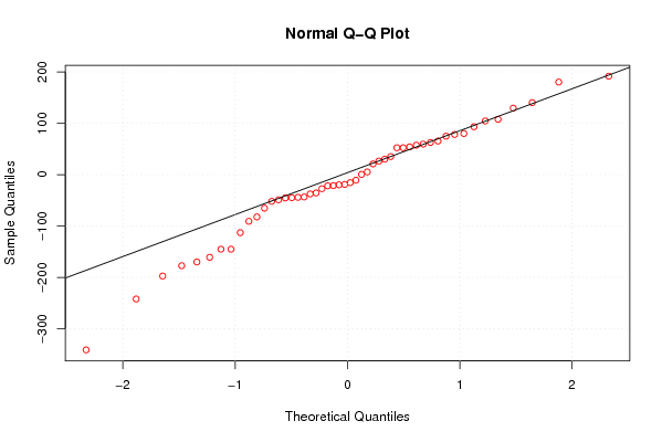
Title produced by software

Percentiles

Date of computation

Thu, 03 Dec 2009 03:35:08 -0700

Cite this page as follows

Statistical Computations at FreeStatistics.org, Office for Research Development and Education, URL https://freestatistics.org/blog/index.php?v=date/2009/Dec/03/t1259836817z1ve5psxxm8xhsv.htm/, Retrieved Sat, 20 Apr 2024 11:55:10 +0000

Statistical Computations at FreeStatistics.org, Office for Research Development and Education, URL https://freestatistics.org/blog/index.php?pk=62673, Retrieved Sat, 20 Apr 2024 11:55:10 +0000

QR Codes:

Paste this QR Code to cite your computation.

Original text written by user:

IsPrivate?

No (this computation is public)

User-defined keywords

Estimated Impact

162

Family? (F = Feedback message, R = changed R code, M = changed R Module, P = changed Parameters, D = changed Data)

-     [Univariate Explorative Data Analysis] [Run Sequence gebo...] [2008-12-12 13:32:37] [76963dc1903f0f612b6153510a3818cf]
- R  D  [Univariate Explorative Data Analysis] [Run Sequence gebo...] [2008-12-17 12:14:40] [76963dc1903f0f612b6153510a3818cf]
-         [Univariate Explorative Data Analysis] [Run Sequence Plot...] [2008-12-22 18:19:51] [1ce0d16c8f4225c977b42c8fa93bc163]
- RMP       [Univariate Data Series] [Identifying Integ...] [2009-11-22 12:08:06] [b98453cac15ba1066b407e146608df68]
- RMPD          [Percentiles] [] [2009-12-03 10:35:08] [2ecea65fec1cd5f6b1ab182881aa2a91] [Current]
-    D            [Percentiles] [] [2009-12-03 17:22:23] [ee35698a38947a6c6c039b1e3deafc05] 
- RMPD              [Harrell-Davis Quantiles] [] [2009-12-04 18:29:06] [eba9b8a72d680086d9ebbb043233c887] 
- RMPD              [Harrell-Davis Quantiles] [] [2009-12-04 18:35:49] [eba9b8a72d680086d9ebbb043233c887] 

Feedback Forum

Post a new message

Dataseries X:

Download CSV

Histogram

Boxplots

0.528987744332542 
-15.5949582292099 
-82.2772184802226 
-197.357097481637 
26.3974003409462 
-45.4166961584019 
-65.2852205280174 
140.189885607142 
52.4365348211837 
93.3428838473187 
104.539808154026 
-44.7673952558717 
-160.840633797359 
80.1272165940445 
57.4266162110635 
54.0628950969678 
74.917288461435 
-10.7437882841881 
35.1953773033078 
180.286871182611 
65.3724560492448 
-341.162457347529 
62.6275190621584 
20.9140594439536 
30.1104507602168 
129.484020098147 
191.702276709734 
-90.851529991777 
-43.5229635161520 
-112.963900079785 
52.3544922133827 
-19.8407136996347 
-169.944452188097 
59.4733519005465 
-177.266106761765 
78.2230945119437 
-21.7654647584984 
-44.0870955597828 
-37.5607005529563 
-145.106051847255 
-35.6395161364094 
-21.3293917666952 
107.778157134319 
-242.014219131835 
-27.3607740313429 
-48.9470850172965 
-51.9695903865187 
-145.095777881986 
5.32431484970925 
-19.0060019212593

Summary of computational transaction
Raw Input	view raw input (R code)
Raw Output	view raw output of R engine
Computing time	1 seconds
R Server	'Gwilym Jenkins' @ 72.249.127.135

\begin{tabular}{lllllllll}
\hline
Summary of computational transaction \tabularnewline
Raw Input & view raw input (R code)  \tabularnewline
Raw Output & view raw output of R engine  \tabularnewline
Computing time & 1 seconds \tabularnewline
R Server & 'Gwilym Jenkins' @ 72.249.127.135 \tabularnewline
\hline
\end{tabular}
%Source: https://freestatistics.org/blog/index.php?pk=62673&T=0

[TABLE]
[ROW][C]Summary of computational transaction[/C][/ROW]
[ROW][C]Raw Input[/C][C]view raw input (R code) [/C][/ROW]
[ROW][C]Raw Output[/C][C]view raw output of R engine [/C][/ROW]
[ROW][C]Computing time[/C][C]1 seconds[/C][/ROW]
[ROW][C]R Server[/C][C]'Gwilym Jenkins' @ 72.249.127.135[/C][/ROW]
[/TABLE]
Source: https://freestatistics.org/blog/index.php?pk=62673&T=0

Globally Unique Identifier (entire table): ba.freestatistics.org/blog/index.php?pk=62673&T=0

As an alternative you can also use a QR Code:

The GUIDs for individual cells are displayed in the table below:

Summary of computational transaction
Raw Input	view raw input (R code)
Raw Output	view raw output of R engine
Computing time	1 seconds
R Server	'Gwilym Jenkins' @ 72.249.127.135

Percentiles - Ungrouped Data
p	Weighted Average at Xnp	Weighted Average at X(n+1)p	Empirical Distribution Function	Empirical Distribution Function - Averaging	Empirical Distribution Function - Interpolation	Closest Observation	True Basic - Statistics Graphics Toolkit	MS Excel (old versions)
0.05	-219.685658	-217.452802	-197.357097	-197.357097	-188.316152	-197.357097	-221.918514	-197.357097
0.1	-169.944452	-169.03407	-169.944452	-165.392543	-161.751016	-169.944452	-161.751016	-169.944452
0.15	-145.100915	-145.099374	-145.095778	-145.095778	-133.849621	-145.095778	-145.102456	-145.095778
0.2	-90.85153	-89.136668	-90.85153	-86.564374	-83.992081	-90.85153	-83.992081	-90.85153
0.25	-58.627405	-55.298498	-51.96959	-51.96959	-51.213964	-51.96959	-61.956313	-51.96959
0.3	-45.416696	-45.221906	-45.416696	-45.092046	-44.962186	-45.416696	-44.962186	-45.416696
0.35	-43.80503	-43.607583	-43.522964	-43.522964	-42.628624	-43.522964	-44.002476	-43.522964
0.4	-35.639516	-32.328019	-35.639516	-31.500145	-30.672271	-35.639516	-30.672271	-35.639516
0.45	-21.547428	-21.351195	-21.329392	-21.329392	-21.254958	-21.329392	-21.743661	-21.329392
0.5	-19.006002	-17.30048	-19.006002	-17.30048	-17.30048	-19.006002	-17.30048	-17.30048
0.55	-5.1074	0.768754	0.528988	0.528988	-0.034651	0.528988	5.084548	0.528988
0.6	20.914059	24.204064	20.914059	23.65573	23.107396	20.914059	23.107396	26.3974
0.65	32.652914	37.769245	35.195377	35.195377	34.432638	35.195377	49.780625	35.195377
0.7	52.436535	53.574987	52.436535	53.249715	52.924443	52.436535	52.924443	54.062895
0.75	58.449984	60.261894	59.473352	59.473352	58.961668	59.473352	61.838977	59.473352
0.8	65.372456	73.008322	65.372456	70.144872	67.281423	65.372456	67.281423	74.917288
0.85	79.175156	84.7527	80.127217	80.127217	79.460774	80.127217	88.7174	80.127217
0.9	104.539808	107.454322	104.539808	106.158983	104.863643	104.539808	104.863643	107.778157
0.95	134.836953	158.233529	140.189886	140.189886	135.372246	140.189886	162.243228	140.189886

\begin{tabular}{lllllllll}
\hline
Percentiles - Ungrouped Data \tabularnewline
p & Weighted Average at Xnp & Weighted Average at X(n+1)p & Empirical Distribution Function & Empirical Distribution Function - Averaging & Empirical Distribution Function - Interpolation & Closest Observation & True Basic - Statistics Graphics Toolkit & MS Excel (old versions) \tabularnewline
0.05 & -219.685658 & -217.452802 & -197.357097 & -197.357097 & -188.316152 & -197.357097 & -221.918514 & -197.357097 \tabularnewline
0.1 & -169.944452 & -169.03407 & -169.944452 & -165.392543 & -161.751016 & -169.944452 & -161.751016 & -169.944452 \tabularnewline
0.15 & -145.100915 & -145.099374 & -145.095778 & -145.095778 & -133.849621 & -145.095778 & -145.102456 & -145.095778 \tabularnewline
0.2 & -90.85153 & -89.136668 & -90.85153 & -86.564374 & -83.992081 & -90.85153 & -83.992081 & -90.85153 \tabularnewline
0.25 & -58.627405 & -55.298498 & -51.96959 & -51.96959 & -51.213964 & -51.96959 & -61.956313 & -51.96959 \tabularnewline
0.3 & -45.416696 & -45.221906 & -45.416696 & -45.092046 & -44.962186 & -45.416696 & -44.962186 & -45.416696 \tabularnewline
0.35 & -43.80503 & -43.607583 & -43.522964 & -43.522964 & -42.628624 & -43.522964 & -44.002476 & -43.522964 \tabularnewline
0.4 & -35.639516 & -32.328019 & -35.639516 & -31.500145 & -30.672271 & -35.639516 & -30.672271 & -35.639516 \tabularnewline
0.45 & -21.547428 & -21.351195 & -21.329392 & -21.329392 & -21.254958 & -21.329392 & -21.743661 & -21.329392 \tabularnewline
0.5 & -19.006002 & -17.30048 & -19.006002 & -17.30048 & -17.30048 & -19.006002 & -17.30048 & -17.30048 \tabularnewline
0.55 & -5.1074 & 0.768754 & 0.528988 & 0.528988 & -0.034651 & 0.528988 & 5.084548 & 0.528988 \tabularnewline
0.6 & 20.914059 & 24.204064 & 20.914059 & 23.65573 & 23.107396 & 20.914059 & 23.107396 & 26.3974 \tabularnewline
0.65 & 32.652914 & 37.769245 & 35.195377 & 35.195377 & 34.432638 & 35.195377 & 49.780625 & 35.195377 \tabularnewline
0.7 & 52.436535 & 53.574987 & 52.436535 & 53.249715 & 52.924443 & 52.436535 & 52.924443 & 54.062895 \tabularnewline
0.75 & 58.449984 & 60.261894 & 59.473352 & 59.473352 & 58.961668 & 59.473352 & 61.838977 & 59.473352 \tabularnewline
0.8 & 65.372456 & 73.008322 & 65.372456 & 70.144872 & 67.281423 & 65.372456 & 67.281423 & 74.917288 \tabularnewline
0.85 & 79.175156 & 84.7527 & 80.127217 & 80.127217 & 79.460774 & 80.127217 & 88.7174 & 80.127217 \tabularnewline
0.9 & 104.539808 & 107.454322 & 104.539808 & 106.158983 & 104.863643 & 104.539808 & 104.863643 & 107.778157 \tabularnewline
0.95 & 134.836953 & 158.233529 & 140.189886 & 140.189886 & 135.372246 & 140.189886 & 162.243228 & 140.189886 \tabularnewline
\hline
\end{tabular}
%Source: https://freestatistics.org/blog/index.php?pk=62673&T=1

[TABLE]
[ROW][C]Percentiles - Ungrouped Data[/C][/ROW]
[ROW][C]p[/C][C]Weighted Average at Xnp[/C][C]Weighted Average at X(n+1)p[/C][C]Empirical Distribution Function[/C][C]Empirical Distribution Function - Averaging[/C][C]Empirical Distribution Function - Interpolation[/C][C]Closest Observation[/C][C]True Basic - Statistics Graphics Toolkit[/C][C]MS Excel (old versions)[/C][/ROW]
[ROW][C]0.05[/C][C]-219.685658[/C][C]-217.452802[/C][C]-197.357097[/C][C]-197.357097[/C][C]-188.316152[/C][C]-197.357097[/C][C]-221.918514[/C][C]-197.357097[/C][/ROW]
[ROW][C]0.1[/C][C]-169.944452[/C][C]-169.03407[/C][C]-169.944452[/C][C]-165.392543[/C][C]-161.751016[/C][C]-169.944452[/C][C]-161.751016[/C][C]-169.944452[/C][/ROW]
[ROW][C]0.15[/C][C]-145.100915[/C][C]-145.099374[/C][C]-145.095778[/C][C]-145.095778[/C][C]-133.849621[/C][C]-145.095778[/C][C]-145.102456[/C][C]-145.095778[/C][/ROW]
[ROW][C]0.2[/C][C]-90.85153[/C][C]-89.136668[/C][C]-90.85153[/C][C]-86.564374[/C][C]-83.992081[/C][C]-90.85153[/C][C]-83.992081[/C][C]-90.85153[/C][/ROW]
[ROW][C]0.25[/C][C]-58.627405[/C][C]-55.298498[/C][C]-51.96959[/C][C]-51.96959[/C][C]-51.213964[/C][C]-51.96959[/C][C]-61.956313[/C][C]-51.96959[/C][/ROW]
[ROW][C]0.3[/C][C]-45.416696[/C][C]-45.221906[/C][C]-45.416696[/C][C]-45.092046[/C][C]-44.962186[/C][C]-45.416696[/C][C]-44.962186[/C][C]-45.416696[/C][/ROW]
[ROW][C]0.35[/C][C]-43.80503[/C][C]-43.607583[/C][C]-43.522964[/C][C]-43.522964[/C][C]-42.628624[/C][C]-43.522964[/C][C]-44.002476[/C][C]-43.522964[/C][/ROW]
[ROW][C]0.4[/C][C]-35.639516[/C][C]-32.328019[/C][C]-35.639516[/C][C]-31.500145[/C][C]-30.672271[/C][C]-35.639516[/C][C]-30.672271[/C][C]-35.639516[/C][/ROW]
[ROW][C]0.45[/C][C]-21.547428[/C][C]-21.351195[/C][C]-21.329392[/C][C]-21.329392[/C][C]-21.254958[/C][C]-21.329392[/C][C]-21.743661[/C][C]-21.329392[/C][/ROW]
[ROW][C]0.5[/C][C]-19.006002[/C][C]-17.30048[/C][C]-19.006002[/C][C]-17.30048[/C][C]-17.30048[/C][C]-19.006002[/C][C]-17.30048[/C][C]-17.30048[/C][/ROW]
[ROW][C]0.55[/C][C]-5.1074[/C][C]0.768754[/C][C]0.528988[/C][C]0.528988[/C][C]-0.034651[/C][C]0.528988[/C][C]5.084548[/C][C]0.528988[/C][/ROW]
[ROW][C]0.6[/C][C]20.914059[/C][C]24.204064[/C][C]20.914059[/C][C]23.65573[/C][C]23.107396[/C][C]20.914059[/C][C]23.107396[/C][C]26.3974[/C][/ROW]
[ROW][C]0.65[/C][C]32.652914[/C][C]37.769245[/C][C]35.195377[/C][C]35.195377[/C][C]34.432638[/C][C]35.195377[/C][C]49.780625[/C][C]35.195377[/C][/ROW]
[ROW][C]0.7[/C][C]52.436535[/C][C]53.574987[/C][C]52.436535[/C][C]53.249715[/C][C]52.924443[/C][C]52.436535[/C][C]52.924443[/C][C]54.062895[/C][/ROW]
[ROW][C]0.75[/C][C]58.449984[/C][C]60.261894[/C][C]59.473352[/C][C]59.473352[/C][C]58.961668[/C][C]59.473352[/C][C]61.838977[/C][C]59.473352[/C][/ROW]
[ROW][C]0.8[/C][C]65.372456[/C][C]73.008322[/C][C]65.372456[/C][C]70.144872[/C][C]67.281423[/C][C]65.372456[/C][C]67.281423[/C][C]74.917288[/C][/ROW]
[ROW][C]0.85[/C][C]79.175156[/C][C]84.7527[/C][C]80.127217[/C][C]80.127217[/C][C]79.460774[/C][C]80.127217[/C][C]88.7174[/C][C]80.127217[/C][/ROW]
[ROW][C]0.9[/C][C]104.539808[/C][C]107.454322[/C][C]104.539808[/C][C]106.158983[/C][C]104.863643[/C][C]104.539808[/C][C]104.863643[/C][C]107.778157[/C][/ROW]
[ROW][C]0.95[/C][C]134.836953[/C][C]158.233529[/C][C]140.189886[/C][C]140.189886[/C][C]135.372246[/C][C]140.189886[/C][C]162.243228[/C][C]140.189886[/C][/ROW]
[/TABLE]
Source: https://freestatistics.org/blog/index.php?pk=62673&T=1

Globally Unique Identifier (entire table): ba.freestatistics.org/blog/index.php?pk=62673&T=1

As an alternative you can also use a QR Code:

The GUIDs for individual cells are displayed in the table below:

Percentiles - Ungrouped Data
p	Weighted Average at Xnp	Weighted Average at X(n+1)p	Empirical Distribution Function	Empirical Distribution Function - Averaging	Empirical Distribution Function - Interpolation	Closest Observation	True Basic - Statistics Graphics Toolkit	MS Excel (old versions)
0.05	-219.685658	-217.452802	-197.357097	-197.357097	-188.316152	-197.357097	-221.918514	-197.357097
0.1	-169.944452	-169.03407	-169.944452	-165.392543	-161.751016	-169.944452	-161.751016	-169.944452
0.15	-145.100915	-145.099374	-145.095778	-145.095778	-133.849621	-145.095778	-145.102456	-145.095778
0.2	-90.85153	-89.136668	-90.85153	-86.564374	-83.992081	-90.85153	-83.992081	-90.85153
0.25	-58.627405	-55.298498	-51.96959	-51.96959	-51.213964	-51.96959	-61.956313	-51.96959
0.3	-45.416696	-45.221906	-45.416696	-45.092046	-44.962186	-45.416696	-44.962186	-45.416696
0.35	-43.80503	-43.607583	-43.522964	-43.522964	-42.628624	-43.522964	-44.002476	-43.522964
0.4	-35.639516	-32.328019	-35.639516	-31.500145	-30.672271	-35.639516	-30.672271	-35.639516
0.45	-21.547428	-21.351195	-21.329392	-21.329392	-21.254958	-21.329392	-21.743661	-21.329392
0.5	-19.006002	-17.30048	-19.006002	-17.30048	-17.30048	-19.006002	-17.30048	-17.30048
0.55	-5.1074	0.768754	0.528988	0.528988	-0.034651	0.528988	5.084548	0.528988
0.6	20.914059	24.204064	20.914059	23.65573	23.107396	20.914059	23.107396	26.3974
0.65	32.652914	37.769245	35.195377	35.195377	34.432638	35.195377	49.780625	35.195377
0.7	52.436535	53.574987	52.436535	53.249715	52.924443	52.436535	52.924443	54.062895
0.75	58.449984	60.261894	59.473352	59.473352	58.961668	59.473352	61.838977	59.473352
0.8	65.372456	73.008322	65.372456	70.144872	67.281423	65.372456	67.281423	74.917288
0.85	79.175156	84.7527	80.127217	80.127217	79.460774	80.127217	88.7174	80.127217
0.9	104.539808	107.454322	104.539808	106.158983	104.863643	104.539808	104.863643	107.778157
0.95	134.836953	158.233529	140.189886	140.189886	135.372246	140.189886	162.243228	140.189886

Figure 1

PNG link

Postscript link

PDF link

Parameters (Session):

Parameters (R input):

R code (references can be found in the software module):

x <-sort(x[!is.na(x)])
q1 <- function(data,n,p,i,f) {
np <- n*p;
i <<- floor(np)
f <<- np - i
qvalue <- (1-f)*data[i] + f*data[i+1]
}
q2 <- function(data,n,p,i,f) {
np <- (n+1)*p
i <<- floor(np)
f <<- np - i
qvalue <- (1-f)*data[i] + f*data[i+1]
}
q3 <- function(data,n,p,i,f) {
np <- n*p
i <<- floor(np)
f <<- np - i
if (f==0) {
qvalue <- data[i]
} else {
qvalue <- data[i+1]
}
}
q4 <- function(data,n,p,i,f) {
np <- n*p
i <<- floor(np)
f <<- np - i
if (f==0) {
qvalue <- (data[i]+data[i+1])/2
} else {
qvalue <- data[i+1]
}
}
q5 <- function(data,n,p,i,f) {
np <- (n-1)*p
i <<- floor(np)
f <<- np - i
if (f==0) {
qvalue <- data[i+1]
} else {
qvalue <- data[i+1] + f*(data[i+2]-data[i+1])
}
}
q6 <- function(data,n,p,i,f) {
np <- n*p+0.5
i <<- floor(np)
f <<- np - i
qvalue <- data[i]
}
q7 <- function(data,n,p,i,f) {
np <- (n+1)*p
i <<- floor(np)
f <<- np - i
if (f==0) {
qvalue <- data[i]
} else {
qvalue <- f*data[i] + (1-f)*data[i+1]
}
}
q8 <- function(data,n,p,i,f) {
np <- (n+1)*p
i <<- floor(np)
f <<- np - i
if (f==0) {
qvalue <- data[i]
} else {
if (f == 0.5) {
qvalue <- (data[i]+data[i+1])/2
} else {
if (f < 0.5) {
qvalue <- data[i]
} else {
qvalue <- data[i+1]
}
}
}
}
lx <- length(x)
qval <- array(NA,dim=c(99,8))
mystep <- 25
mystart <- 25
if (lx>10){
mystep=10
mystart=10
}
if (lx>20){
mystep=5
mystart=5
}
if (lx>50){
mystep=2
mystart=2
}
if (lx>=100){
mystep=1
mystart=1
}
for (perc in seq(mystart,99,mystep)) {
qval[perc,1] <- q1(x,lx,perc/100,i,f)
qval[perc,2] <- q2(x,lx,perc/100,i,f)
qval[perc,3] <- q3(x,lx,perc/100,i,f)
qval[perc,4] <- q4(x,lx,perc/100,i,f)
qval[perc,5] <- q5(x,lx,perc/100,i,f)
qval[perc,6] <- q6(x,lx,perc/100,i,f)
qval[perc,7] <- q7(x,lx,perc/100,i,f)
qval[perc,8] <- q8(x,lx,perc/100,i,f)
}
bitmap(file='test1.png')
myqqnorm <- qqnorm(x,col=2)
qqline(x)
grid()
dev.off()
load(file='createtable')
a<-table.start()
a<-table.row.start(a)
a<-table.element(a,'Percentiles - Ungrouped Data',9,TRUE)
a<-table.row.end(a)
a<-table.row.start(a)
a<-table.element(a,'p',1,TRUE)
a<-table.element(a,hyperlink('method_1.htm', 'Weighted Average at Xnp',''),1,TRUE)
a<-table.element(a,hyperlink('method_2.htm','Weighted Average at X(n+1)p',''),1,TRUE)
a<-table.element(a,hyperlink('method_3.htm','Empirical Distribution Function',''),1,TRUE)
a<-table.element(a,hyperlink('method_4.htm','Empirical Distribution Function - Averaging',''),1,TRUE)
a<-table.element(a,hyperlink('method_5.htm','Empirical Distribution Function - Interpolation',''),1,TRUE)
a<-table.element(a,hyperlink('method_6.htm','Closest Observation',''),1,TRUE)
a<-table.element(a,hyperlink('method_7.htm','True Basic - Statistics Graphics Toolkit',''),1,TRUE)
a<-table.element(a,hyperlink('method_8.htm','MS Excel (old versions)',''),1,TRUE)
a<-table.row.end(a)
for (perc in seq(mystart,99,mystep)) {
a<-table.row.start(a)
a<-table.element(a,round(perc/100,2),1,TRUE)
for (j in 1:8) {
a<-table.element(a,round(qval[perc,j],6))
}
a<-table.row.end(a)
}
a<-table.end(a)
table.save(a,file='mytable.tab')

Free Statistics

Description of Statistical Computation

Tree of Dependent Computations

Dataset

Tables (Output of Computation)

Figures (Output of Computation)

Input Parameters & R Code