Free Statistics
of Irreproducible Research!
Description of Statistical Computation | |||||||||||||||||||||
|---|---|---|---|---|---|---|---|---|---|---|---|---|---|---|---|---|---|---|---|---|---|
| Author's title | |||||||||||||||||||||
| Author | *The author of this computation has been verified* | ||||||||||||||||||||
| R Software Module | rwasp_meanplot.wasp | ||||||||||||||||||||
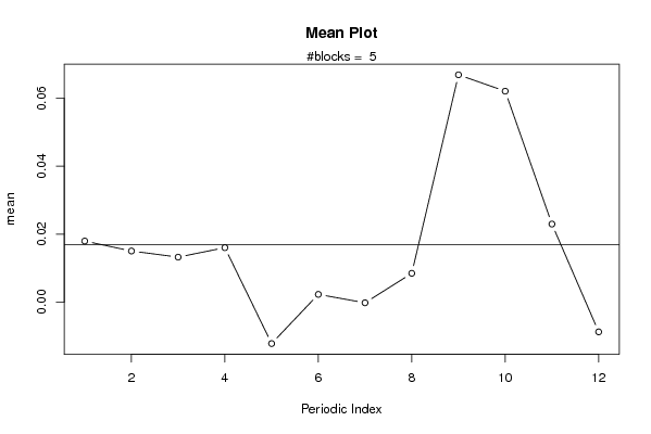
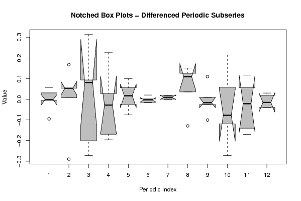
| Title produced by software | Mean Plot | ||||||||||||||||||||
| Date of computation | Tue, 01 Dec 2009 14:28:00 -0700 | ||||||||||||||||||||
| Cite this page as follows | Statistical Computations at FreeStatistics.org, Office for Research Development and Education, URL https://freestatistics.org/blog/index.php?v=date/2009/Dec/01/t1259702933dbpj02ekx5w4pej.htm/, Retrieved Sat, 27 Apr 2024 04:49:50 +0000 | ||||||||||||||||||||
| Statistical Computations at FreeStatistics.org, Office for Research Development and Education, URL https://freestatistics.org/blog/index.php?pk=62269, Retrieved Sat, 27 Apr 2024 04:49:50 +0000 | |||||||||||||||||||||
| QR Codes: | |||||||||||||||||||||
|
| |||||||||||||||||||||
| Original text written by user: | |||||||||||||||||||||
| IsPrivate? | No (this computation is public) | ||||||||||||||||||||
| User-defined keywords | |||||||||||||||||||||
| Estimated Impact | 145 | ||||||||||||||||||||
Tree of Dependent Computations | |||||||||||||||||||||
| Family? (F = Feedback message, R = changed R code, M = changed R Module, P = changed Parameters, D = changed Data) | |||||||||||||||||||||
| - [Kendall tau Correlation Matrix] [Correlatie tussen...] [2007-11-03 21:44:17] [0b2d8ed757c467aee7199cdee05779c9] - RMPD [(Partial) Autocorrelation Function] [WS 8 01] [2009-11-21 08:59:55] [6e4e01d7eb22a9f33d58ebb35753a195] - PD [(Partial) Autocorrelation Function] [WS 8 02] [2009-11-21 11:01:08] [6e4e01d7eb22a9f33d58ebb35753a195] - P [(Partial) Autocorrelation Function] [WS 8 03] [2009-11-21 11:02:54] [6e4e01d7eb22a9f33d58ebb35753a195] - P [(Partial) Autocorrelation Function] [ws9] [2009-11-29 12:25:47] [6e4e01d7eb22a9f33d58ebb35753a195] - RMPD [Mean Plot] [ws 9 m] [2009-12-01 21:28:00] [2e4ef2c1b76db9b31c0a03b96e94ad77] [Current] | |||||||||||||||||||||
| Feedback Forum | |||||||||||||||||||||
Post a new message | |||||||||||||||||||||
Dataset | |||||||||||||||||||||
| Dataseries X: | |||||||||||||||||||||
0.103629933239820 0.0087703074390444 0.0155637426660695 0.0966084256018938 0.0683025606568869 -0.00653314961359896 -0.0094367257568807 0.00935003832683242 0.118449494805129 0.127456615819888 0.00876382231245558 -0.0129824429665246 -0.00415418317902038 0.0266421877779411 0.194032448777481 -0.00711070355878007 0.0205688036309368 -0.00442856389169322 -0.00315893309607418 0.0064652048591256 0.131873973578195 0.241305044412940 -0.0310262850916416 0.0245251063758616 -0.0156222322911219 -0.0206043854226294 0.0326967759710612 0.125988059619388 -0.0435502067574021 0.0123515713707718 -0.00434737918082817 -0.00353479514087951 0.147562133549002 0.0470693504162938 0.105815471844778 -0.0341342674195459 -0.00414417660174138 -0.0064652048591256 0.0468257381816528 -0.225104141948705 3.12331458758308e-05 0.0166685620235825 0.00237689216950798 0 0.0357693020416008 0.0102083822537082 -0.0675670602819736 0.0495991980182566 0.0101167955535715 0.0668105237905223 -0.223001756937975 0.0896858022691731 -0.106531513400583 -0.00678504840645644 0.0134485427007007 0.0300000000000011 -0.0989691535751547 -0.115464366100554 0.0988679532745067 -0.0709498589393718 | |||||||||||||||||||||
Tables (Output of Computation) | |||||||||||||||||||||
| |||||||||||||||||||||
Figures (Output of Computation) | |||||||||||||||||||||
Input Parameters & R Code | |||||||||||||||||||||
| Parameters (Session): | |||||||||||||||||||||
| par1 = 12 ; | |||||||||||||||||||||
| Parameters (R input): | |||||||||||||||||||||
| par1 = 12 ; | |||||||||||||||||||||
| R code (references can be found in the software module): | |||||||||||||||||||||
par1 <- as.numeric(par1) | |||||||||||||||||||||