Free Statistics
of Irreproducible Research!
Description of Statistical Computation | |||||||||||||||||||||
|---|---|---|---|---|---|---|---|---|---|---|---|---|---|---|---|---|---|---|---|---|---|
| Author's title | |||||||||||||||||||||
| Author | *The author of this computation has been verified* | ||||||||||||||||||||
| R Software Module | rwasp_meanplot.wasp | ||||||||||||||||||||
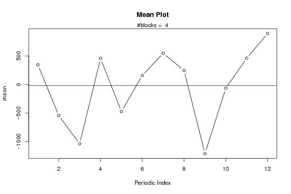
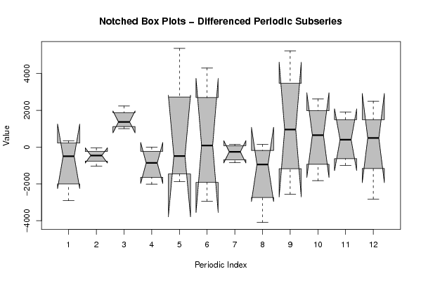
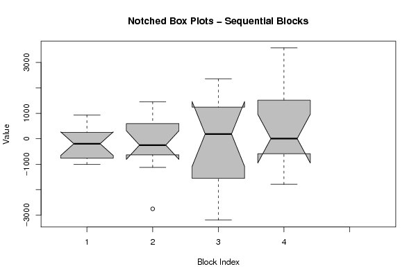
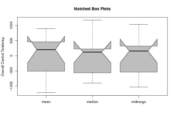
| Title produced by software | Mean Plot | ||||||||||||||||||||
| Date of computation | Tue, 01 Dec 2009 12:01:30 -0700 | ||||||||||||||||||||
| Cite this page as follows | Statistical Computations at FreeStatistics.org, Office for Research Development and Education, URL https://freestatistics.org/blog/index.php?v=date/2009/Dec/01/t1259694281elpntyqfue6ywhd.htm/, Retrieved Wed, 24 Apr 2024 12:06:45 +0000 | ||||||||||||||||||||
| Statistical Computations at FreeStatistics.org, Office for Research Development and Education, URL https://freestatistics.org/blog/index.php?pk=62192, Retrieved Wed, 24 Apr 2024 12:06:45 +0000 | |||||||||||||||||||||
| QR Codes: | |||||||||||||||||||||
|
| |||||||||||||||||||||
| Original text written by user: | |||||||||||||||||||||
| IsPrivate? | No (this computation is public) | ||||||||||||||||||||
| User-defined keywords | |||||||||||||||||||||
| Estimated Impact | 171 | ||||||||||||||||||||
Tree of Dependent Computations | |||||||||||||||||||||
| Family? (F = Feedback message, R = changed R code, M = changed R Module, P = changed Parameters, D = changed Data) | |||||||||||||||||||||
| - [Univariate Data Series] [data set] [2008-12-01 19:54:57] [b98453cac15ba1066b407e146608df68] - RMP [ARIMA Backward Selection] [] [2009-11-27 14:53:14] [b98453cac15ba1066b407e146608df68] - RMPD [Mean Plot] [] [2009-12-01 19:01:30] [7dd0431c761b876151627bfbf92230c8] [Current] | |||||||||||||||||||||
| Feedback Forum | |||||||||||||||||||||
Post a new message | |||||||||||||||||||||
Dataset | |||||||||||||||||||||
| Dataseries X: | |||||||||||||||||||||
-319.559557390785 27.9743410117227 -1008.46959533542 219.863126270784 -234.491311787668 -153.082960538935 933.953124451168 411.042384090291 -961.89720235503 -744.764396776115 -784.92892986467 290.509724746436 785.730745077288 -301.538747036842 -780.030839489239 1454.61282130082 1455.43851042382 411.425730256672 -489.069183914927 -338.63085750037 -193.728983946927 -2756.28930305837 -138.899095490555 -1123.79015926020 1375.20173898251 -1535.1755035624 -1580.22317024033 -64.5953189787947 -1328.41699726220 -3198.05965476559 1102.44538925562 1119.07222818829 -2973.61872170023 2265.07317206589 443.326906414096 2358.41463625693 -459.228166651762 -366.686092276445 -788.24933923038 221.857682470493 -1789.68439905851 3575.1307429011 639.708861362199 -209.773692601329 -713.751966817262 979.24918300219 2326.97019964138 2055.60615831213 | |||||||||||||||||||||
Tables (Output of Computation) | |||||||||||||||||||||
| |||||||||||||||||||||
Figures (Output of Computation) | |||||||||||||||||||||
Input Parameters & R Code | |||||||||||||||||||||
| Parameters (Session): | |||||||||||||||||||||
| par1 = 12 ; | |||||||||||||||||||||
| Parameters (R input): | |||||||||||||||||||||
| par1 = 12 ; | |||||||||||||||||||||
| R code (references can be found in the software module): | |||||||||||||||||||||
par1 <- as.numeric(par1) | |||||||||||||||||||||