Free Statistics
of Irreproducible Research!
Description of Statistical Computation | |||||||||||||||||||||
|---|---|---|---|---|---|---|---|---|---|---|---|---|---|---|---|---|---|---|---|---|---|
| Author's title | |||||||||||||||||||||
| Author | *Unverified author* | ||||||||||||||||||||
| R Software Module | rwasp_meanplot.wasp | ||||||||||||||||||||
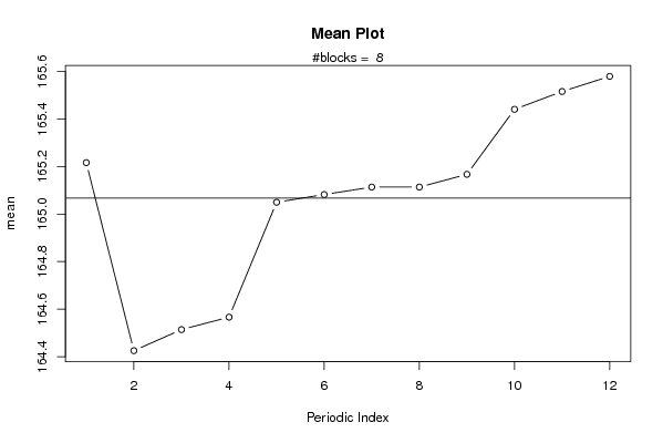
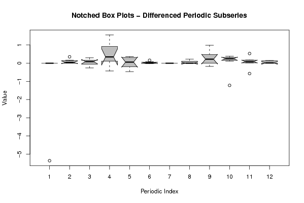
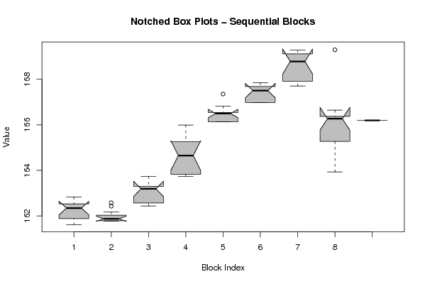
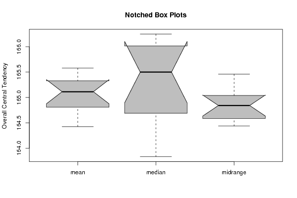
| Title produced by software | Mean Plot | ||||||||||||||||||||
| Date of computation | Tue, 01 Dec 2009 10:52:07 -0700 | ||||||||||||||||||||
| Cite this page as follows | Statistical Computations at FreeStatistics.org, Office for Research Development and Education, URL https://freestatistics.org/blog/index.php?v=date/2009/Dec/01/t1259690216pvch0xkyo5yo05l.htm/, Retrieved Fri, 26 Apr 2024 03:58:46 +0000 | ||||||||||||||||||||
| Statistical Computations at FreeStatistics.org, Office for Research Development and Education, URL https://freestatistics.org/blog/index.php?pk=62152, Retrieved Fri, 26 Apr 2024 03:58:46 +0000 | |||||||||||||||||||||
| QR Codes: | |||||||||||||||||||||
|
| |||||||||||||||||||||
| Original text written by user: | |||||||||||||||||||||
| IsPrivate? | No (this computation is public) | ||||||||||||||||||||
| User-defined keywords | Mean plot gemiddelde blazer | ||||||||||||||||||||
| Estimated Impact | 157 | ||||||||||||||||||||
Tree of Dependent Computations | |||||||||||||||||||||
| Family? (F = Feedback message, R = changed R code, M = changed R Module, P = changed Parameters, D = changed Data) | |||||||||||||||||||||
| - [Univariate Data Series] [Gemiddelde prijs ...] [2009-09-22 17:16:52] [101768e0846f790d4a51eca83c4a4208] - RMPD [Mean Plot] [KDGP2W12] [2009-12-01 17:52:07] [f8fa19533df6d92688ec2c19e4765e3f] [Current] | |||||||||||||||||||||
| Feedback Forum | |||||||||||||||||||||
Post a new message | |||||||||||||||||||||
Dataset | |||||||||||||||||||||
| Dataseries X: | |||||||||||||||||||||
161.88 161.88 162.05 162.16 162.61 162.53 162.53 162.53 162.53 162.83 161.61 161.79 161.79 161.79 161.79 161.85 161.77 161.86 161.89 161.89 161.89 162.18 162.43 162.58 162.57 162.57 162.57 162.44 162.79 163.15 163.23 163.23 163.23 163.38 163.71 163.73 163.73 163.73 163.73 163.93 164.27 164.57 164.73 164.73 164.76 165.75 165.86 165.99 166.13 166.13 166.13 166.15 166.45 166.48 166.51 166.51 166.51 166.58 166.82 167.35 167.5 167.5 167.6 167.72 167.29 166.98 166.98 166.98 166.98 167.63 167.83 167.85 167.87 167.87 167.96 167.7 169.25 168.79 168.77 168.77 169 168.92 169.23 169.28 169.29 163.93 164.28 164.58 165.97 166.3 166.27 166.27 166.44 166.26 166.64 166.07 166.19 | |||||||||||||||||||||
Tables (Output of Computation) | |||||||||||||||||||||
| |||||||||||||||||||||
Figures (Output of Computation) | |||||||||||||||||||||
Input Parameters & R Code | |||||||||||||||||||||
| Parameters (Session): | |||||||||||||||||||||
| par1 = 12 ; | |||||||||||||||||||||
| Parameters (R input): | |||||||||||||||||||||
| par1 = 12 ; | |||||||||||||||||||||
| R code (references can be found in the software module): | |||||||||||||||||||||
par1 <- as.numeric(par1) | |||||||||||||||||||||