Repository of Reproducible Computations

Free Statistics

of Irreproducible Research!

Author's title

Author

*The author of this computation has been verified*

R Software Module

rwasp_autocorrelation.wasp

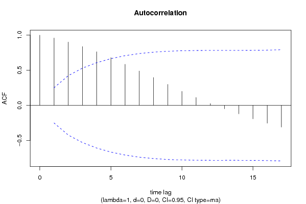
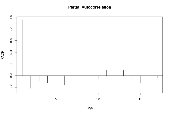
Title produced by software

(Partial) Autocorrelation Function

Date of computation

Tue, 01 Dec 2009 10:11:01 -0700

Cite this page as follows

Statistical Computations at FreeStatistics.org, Office for Research Development and Education, URL https://freestatistics.org/blog/index.php?v=date/2009/Dec/01/t1259687607gndxs5stly7z3nq.htm/, Retrieved Wed, 01 May 2024 21:46:48 +0000

Statistical Computations at FreeStatistics.org, Office for Research Development and Education, URL https://freestatistics.org/blog/index.php?pk=62130, Retrieved Wed, 01 May 2024 21:46:48 +0000

QR Codes:

Paste this QR Code to cite your computation.

Original text written by user:

IsPrivate?

No (this computation is public)

User-defined keywords

Estimated Impact

162

Family? (F = Feedback message, R = changed R code, M = changed R Module, P = changed Parameters, D = changed Data)

-     [Univariate Data Series] [data set] [2008-12-01 19:54:57] [b98453cac15ba1066b407e146608df68]
- RMP   [(Partial) Autocorrelation Function] [] [2009-11-27 14:46:03] [b98453cac15ba1066b407e146608df68]
- R PD      [(Partial) Autocorrelation Function] [] [2009-12-01 17:11:01] [791a4a78a0a7ca497fb8791b982a539e] [Current]
- R  D        [(Partial) Autocorrelation Function] [AutoCF d=0,D=0] [2009-12-04 15:09:00] [fa71ec4c741ffec745cb91dcbd756720] 
-   PD        [(Partial) Autocorrelation Function] [] [2009-12-08 17:32:48] [ee35698a38947a6c6c039b1e3deafc05] 
-   PD        [(Partial) Autocorrelation Function] [] [2009-12-08 17:38:21] [ee35698a38947a6c6c039b1e3deafc05] 
-   P           [(Partial) Autocorrelation Function] [] [2009-12-08 18:08:14] [ee35698a38947a6c6c039b1e3deafc05] 

Feedback Forum

Post a new message

Dataseries X:

Download CSV

Histogram

Boxplots

Summary of computational transaction
Raw Input	view raw input (R code)
Raw Output	view raw output of R engine
Computing time	1 seconds
R Server	'Gwilym Jenkins' @ 72.249.127.135

\begin{tabular}{lllllllll}
\hline
Summary of computational transaction \tabularnewline
Raw Input & view raw input (R code)  \tabularnewline
Raw Output & view raw output of R engine  \tabularnewline
Computing time & 1 seconds \tabularnewline
R Server & 'Gwilym Jenkins' @ 72.249.127.135 \tabularnewline
\hline
\end{tabular}
%Source: https://freestatistics.org/blog/index.php?pk=62130&T=0

[TABLE]
[ROW][C]Summary of computational transaction[/C][/ROW]
[ROW][C]Raw Input[/C][C]view raw input (R code) [/C][/ROW]
[ROW][C]Raw Output[/C][C]view raw output of R engine [/C][/ROW]
[ROW][C]Computing time[/C][C]1 seconds[/C][/ROW]
[ROW][C]R Server[/C][C]'Gwilym Jenkins' @ 72.249.127.135[/C][/ROW]
[/TABLE]
Source: https://freestatistics.org/blog/index.php?pk=62130&T=0

Globally Unique Identifier (entire table): ba.freestatistics.org/blog/index.php?pk=62130&T=0

As an alternative you can also use a QR Code:

The GUIDs for individual cells are displayed in the table below:

Summary of computational transaction
Raw Input	view raw input (R code)
Raw Output	view raw output of R engine
Computing time	1 seconds
R Server	'Gwilym Jenkins' @ 72.249.127.135

Autocorrelation Function
Time lag k	ACF(k)	T-STAT	P-value
1	0.958916	7.4894	0
2	0.901977	7.0447	0
3	0.837422	6.5405	0
4	0.76419	5.9685	0
5	0.680721	5.3166	1e-06
6	0.585479	4.5727	1.2e-05
7	0.489702	3.8247	0.000155
8	0.397003	3.1007	0.001461
9	0.298722	2.3331	0.011478
10	0.199536	1.5584	0.062152
11	0.112319	0.8772	0.1919
12	0.025389	0.1983	0.421736
13	-0.048756	-0.3808	0.352338
14	-0.120594	-0.9419	0.174988
15	-0.192875	-1.5064	0.068562
16	-0.253964	-1.9835	0.025907
17	-0.309141	-2.4145	0.009386

\begin{tabular}{lllllllll}
\hline
Autocorrelation Function \tabularnewline
Time lag k & ACF(k) & T-STAT & P-value \tabularnewline
1 & 0.958916 & 7.4894 & 0 \tabularnewline
2 & 0.901977 & 7.0447 & 0 \tabularnewline
3 & 0.837422 & 6.5405 & 0 \tabularnewline
4 & 0.76419 & 5.9685 & 0 \tabularnewline
5 & 0.680721 & 5.3166 & 1e-06 \tabularnewline
6 & 0.585479 & 4.5727 & 1.2e-05 \tabularnewline
7 & 0.489702 & 3.8247 & 0.000155 \tabularnewline
8 & 0.397003 & 3.1007 & 0.001461 \tabularnewline
9 & 0.298722 & 2.3331 & 0.011478 \tabularnewline
10 & 0.199536 & 1.5584 & 0.062152 \tabularnewline
11 & 0.112319 & 0.8772 & 0.1919 \tabularnewline
12 & 0.025389 & 0.1983 & 0.421736 \tabularnewline
13 & -0.048756 & -0.3808 & 0.352338 \tabularnewline
14 & -0.120594 & -0.9419 & 0.174988 \tabularnewline
15 & -0.192875 & -1.5064 & 0.068562 \tabularnewline
16 & -0.253964 & -1.9835 & 0.025907 \tabularnewline
17 & -0.309141 & -2.4145 & 0.009386 \tabularnewline
\hline
\end{tabular}
%Source: https://freestatistics.org/blog/index.php?pk=62130&T=1

[TABLE]
[ROW][C]Autocorrelation Function[/C][/ROW]
[ROW][C]Time lag k[/C][C]ACF(k)[/C][C]T-STAT[/C][C]P-value[/C][/ROW]
[ROW][C]1[/C][C]0.958916[/C][C]7.4894[/C][C]0[/C][/ROW]
[ROW][C]2[/C][C]0.901977[/C][C]7.0447[/C][C]0[/C][/ROW]
[ROW][C]3[/C][C]0.837422[/C][C]6.5405[/C][C]0[/C][/ROW]
[ROW][C]4[/C][C]0.76419[/C][C]5.9685[/C][C]0[/C][/ROW]
[ROW][C]5[/C][C]0.680721[/C][C]5.3166[/C][C]1e-06[/C][/ROW]
[ROW][C]6[/C][C]0.585479[/C][C]4.5727[/C][C]1.2e-05[/C][/ROW]
[ROW][C]7[/C][C]0.489702[/C][C]3.8247[/C][C]0.000155[/C][/ROW]
[ROW][C]8[/C][C]0.397003[/C][C]3.1007[/C][C]0.001461[/C][/ROW]
[ROW][C]9[/C][C]0.298722[/C][C]2.3331[/C][C]0.011478[/C][/ROW]
[ROW][C]10[/C][C]0.199536[/C][C]1.5584[/C][C]0.062152[/C][/ROW]
[ROW][C]11[/C][C]0.112319[/C][C]0.8772[/C][C]0.1919[/C][/ROW]
[ROW][C]12[/C][C]0.025389[/C][C]0.1983[/C][C]0.421736[/C][/ROW]
[ROW][C]13[/C][C]-0.048756[/C][C]-0.3808[/C][C]0.352338[/C][/ROW]
[ROW][C]14[/C][C]-0.120594[/C][C]-0.9419[/C][C]0.174988[/C][/ROW]
[ROW][C]15[/C][C]-0.192875[/C][C]-1.5064[/C][C]0.068562[/C][/ROW]
[ROW][C]16[/C][C]-0.253964[/C][C]-1.9835[/C][C]0.025907[/C][/ROW]
[ROW][C]17[/C][C]-0.309141[/C][C]-2.4145[/C][C]0.009386[/C][/ROW]
[/TABLE]
Source: https://freestatistics.org/blog/index.php?pk=62130&T=1

Globally Unique Identifier (entire table): ba.freestatistics.org/blog/index.php?pk=62130&T=1

As an alternative you can also use a QR Code:

The GUIDs for individual cells are displayed in the table below:

Autocorrelation Function
Time lag k	ACF(k)	T-STAT	P-value
1	0.958916	7.4894	0
2	0.901977	7.0447	0
3	0.837422	6.5405	0
4	0.76419	5.9685	0
5	0.680721	5.3166	1e-06
6	0.585479	4.5727	1.2e-05
7	0.489702	3.8247	0.000155
8	0.397003	3.1007	0.001461
9	0.298722	2.3331	0.011478
10	0.199536	1.5584	0.062152
11	0.112319	0.8772	0.1919
12	0.025389	0.1983	0.421736
13	-0.048756	-0.3808	0.352338
14	-0.120594	-0.9419	0.174988
15	-0.192875	-1.5064	0.068562
16	-0.253964	-1.9835	0.025907
17	-0.309141	-2.4145	0.009386

Partial Autocorrelation Function
Time lag k	PACF(k)	T-STAT	P-value
1	0.958916	7.4894	0
2	-0.217988	-1.7025	0.046873
3	-0.091425	-0.7141	0.23896
4	-0.121162	-0.9463	0.173862
5	-0.140467	-1.0971	0.138459
6	-0.163897	-1.2801	0.102683
7	-0.015351	-0.1199	0.45248
8	-0.005438	-0.0425	0.483132
9	-0.136438	-1.0656	0.145399
10	-0.057766	-0.4512	0.326736
11	0.091158	0.712	0.239599
12	-0.13205	-1.0313	0.153225
13	0.089274	0.6973	0.244147
14	-0.09243	-0.7219	0.236556
15	-0.130504	-1.0193	0.15605
16	0.020568	0.1606	0.436453
17	-0.046841	-0.3658	0.357874

\begin{tabular}{lllllllll}
\hline
Partial Autocorrelation Function \tabularnewline
Time lag k & PACF(k) & T-STAT & P-value \tabularnewline
1 & 0.958916 & 7.4894 & 0 \tabularnewline
2 & -0.217988 & -1.7025 & 0.046873 \tabularnewline
3 & -0.091425 & -0.7141 & 0.23896 \tabularnewline
4 & -0.121162 & -0.9463 & 0.173862 \tabularnewline
5 & -0.140467 & -1.0971 & 0.138459 \tabularnewline
6 & -0.163897 & -1.2801 & 0.102683 \tabularnewline
7 & -0.015351 & -0.1199 & 0.45248 \tabularnewline
8 & -0.005438 & -0.0425 & 0.483132 \tabularnewline
9 & -0.136438 & -1.0656 & 0.145399 \tabularnewline
10 & -0.057766 & -0.4512 & 0.326736 \tabularnewline
11 & 0.091158 & 0.712 & 0.239599 \tabularnewline
12 & -0.13205 & -1.0313 & 0.153225 \tabularnewline
13 & 0.089274 & 0.6973 & 0.244147 \tabularnewline
14 & -0.09243 & -0.7219 & 0.236556 \tabularnewline
15 & -0.130504 & -1.0193 & 0.15605 \tabularnewline
16 & 0.020568 & 0.1606 & 0.436453 \tabularnewline
17 & -0.046841 & -0.3658 & 0.357874 \tabularnewline
\hline
\end{tabular}
%Source: https://freestatistics.org/blog/index.php?pk=62130&T=2

[TABLE]
[ROW][C]Partial Autocorrelation Function[/C][/ROW]
[ROW][C]Time lag k[/C][C]PACF(k)[/C][C]T-STAT[/C][C]P-value[/C][/ROW]
[ROW][C]1[/C][C]0.958916[/C][C]7.4894[/C][C]0[/C][/ROW]
[ROW][C]2[/C][C]-0.217988[/C][C]-1.7025[/C][C]0.046873[/C][/ROW]
[ROW][C]3[/C][C]-0.091425[/C][C]-0.7141[/C][C]0.23896[/C][/ROW]
[ROW][C]4[/C][C]-0.121162[/C][C]-0.9463[/C][C]0.173862[/C][/ROW]
[ROW][C]5[/C][C]-0.140467[/C][C]-1.0971[/C][C]0.138459[/C][/ROW]
[ROW][C]6[/C][C]-0.163897[/C][C]-1.2801[/C][C]0.102683[/C][/ROW]
[ROW][C]7[/C][C]-0.015351[/C][C]-0.1199[/C][C]0.45248[/C][/ROW]
[ROW][C]8[/C][C]-0.005438[/C][C]-0.0425[/C][C]0.483132[/C][/ROW]
[ROW][C]9[/C][C]-0.136438[/C][C]-1.0656[/C][C]0.145399[/C][/ROW]
[ROW][C]10[/C][C]-0.057766[/C][C]-0.4512[/C][C]0.326736[/C][/ROW]
[ROW][C]11[/C][C]0.091158[/C][C]0.712[/C][C]0.239599[/C][/ROW]
[ROW][C]12[/C][C]-0.13205[/C][C]-1.0313[/C][C]0.153225[/C][/ROW]
[ROW][C]13[/C][C]0.089274[/C][C]0.6973[/C][C]0.244147[/C][/ROW]
[ROW][C]14[/C][C]-0.09243[/C][C]-0.7219[/C][C]0.236556[/C][/ROW]
[ROW][C]15[/C][C]-0.130504[/C][C]-1.0193[/C][C]0.15605[/C][/ROW]
[ROW][C]16[/C][C]0.020568[/C][C]0.1606[/C][C]0.436453[/C][/ROW]
[ROW][C]17[/C][C]-0.046841[/C][C]-0.3658[/C][C]0.357874[/C][/ROW]
[/TABLE]
Source: https://freestatistics.org/blog/index.php?pk=62130&T=2

Globally Unique Identifier (entire table): ba.freestatistics.org/blog/index.php?pk=62130&T=2

As an alternative you can also use a QR Code:

The GUIDs for individual cells are displayed in the table below:

Partial Autocorrelation Function
Time lag k	PACF(k)	T-STAT	P-value
1	0.958916	7.4894	0
2	-0.217988	-1.7025	0.046873
3	-0.091425	-0.7141	0.23896
4	-0.121162	-0.9463	0.173862
5	-0.140467	-1.0971	0.138459
6	-0.163897	-1.2801	0.102683
7	-0.015351	-0.1199	0.45248
8	-0.005438	-0.0425	0.483132
9	-0.136438	-1.0656	0.145399
10	-0.057766	-0.4512	0.326736
11	0.091158	0.712	0.239599
12	-0.13205	-1.0313	0.153225
13	0.089274	0.6973	0.244147
14	-0.09243	-0.7219	0.236556
15	-0.130504	-1.0193	0.15605
16	0.020568	0.1606	0.436453
17	-0.046841	-0.3658	0.357874

Figure 1

PNG link

Postscript link

PDF link

Figure 2

PNG link

Postscript link

PDF link

Parameters (Session):

par1 = Default ; par2 = 1 ; par3 = 0 ; par4 = 0 ; par5 = 12 ; par6 = MA ; par7 = 0.95 ;

Parameters (R input):

par1 = Default ; par2 = 1 ; par3 = 0 ; par4 = 0 ; par5 = 12 ; par6 = MA ; par7 = 0.95 ;

R code (references can be found in the software module):

if (par1 == 'Default') {
par1 = 10*log10(length(x))
} else {
par1 <- as.numeric(par1)
}
par2 <- as.numeric(par2)
par3 <- as.numeric(par3)
par4 <- as.numeric(par4)
par5 <- as.numeric(par5)
if (par6 == 'White Noise') par6 <- 'white' else par6 <- 'ma'
par7 <- as.numeric(par7)
if (par2 == 0) {
x <- log(x)
} else {
x <- (x ^ par2 - 1) / par2
}
if (par3 > 0) x <- diff(x,lag=1,difference=par3)
if (par4 > 0) x <- diff(x,lag=par5,difference=par4)
bitmap(file='pic1.png')
racf <- acf(x, par1, main='Autocorrelation', xlab='time lag', ylab='ACF', ci.type=par6, ci=par7, sub=paste('(lambda=',par2,', d=',par3,', D=',par4,', CI=', par7, ', CI type=',par6,')',sep=''))
dev.off()
bitmap(file='pic2.png')
rpacf <- pacf(x,par1,main='Partial Autocorrelation',xlab='lags',ylab='PACF')
dev.off()
(myacf <- c(racf$acf))
(mypacf <- c(rpacf$acf))
lengthx <- length(x)
sqrtn <- sqrt(lengthx)
load(file='createtable')
a<-table.start()
a<-table.row.start(a)
a<-table.element(a,'Autocorrelation Function',4,TRUE)
a<-table.row.end(a)
a<-table.row.start(a)
a<-table.element(a,'Time lag k',header=TRUE)
a<-table.element(a,hyperlink('basics.htm','ACF(k)','click here for more information about the Autocorrelation Function'),header=TRUE)
a<-table.element(a,'T-STAT',header=TRUE)
a<-table.element(a,'P-value',header=TRUE)
a<-table.row.end(a)
for (i in 2:(par1+1)) {
a<-table.row.start(a)
a<-table.element(a,i-1,header=TRUE)
a<-table.element(a,round(myacf[i],6))
mytstat <- myacf[i]*sqrtn
a<-table.element(a,round(mytstat,4))
a<-table.element(a,round(1-pt(abs(mytstat),lengthx),6))
a<-table.row.end(a)
}
a<-table.end(a)
table.save(a,file='mytable.tab')
a<-table.start()
a<-table.row.start(a)
a<-table.element(a,'Partial Autocorrelation Function',4,TRUE)
a<-table.row.end(a)
a<-table.row.start(a)
a<-table.element(a,'Time lag k',header=TRUE)
a<-table.element(a,hyperlink('basics.htm','PACF(k)','click here for more information about the Partial Autocorrelation Function'),header=TRUE)
a<-table.element(a,'T-STAT',header=TRUE)
a<-table.element(a,'P-value',header=TRUE)
a<-table.row.end(a)
for (i in 1:par1) {
a<-table.row.start(a)
a<-table.element(a,i,header=TRUE)
a<-table.element(a,round(mypacf[i],6))
mytstat <- mypacf[i]*sqrtn
a<-table.element(a,round(mytstat,4))
a<-table.element(a,round(1-pt(abs(mytstat),lengthx),6))
a<-table.row.end(a)
}
a<-table.end(a)
table.save(a,file='mytable1.tab')

Free Statistics

Description of Statistical Computation

Tree of Dependent Computations

Dataset

Tables (Output of Computation)

Figures (Output of Computation)

Input Parameters & R Code