Free Statistics
of Irreproducible Research!
Description of Statistical Computation | |||||||||||||||||||||
|---|---|---|---|---|---|---|---|---|---|---|---|---|---|---|---|---|---|---|---|---|---|
| Author's title | |||||||||||||||||||||
| Author | *Unverified author* | ||||||||||||||||||||
| R Software Module | rwasp_sdplot.wasp | ||||||||||||||||||||
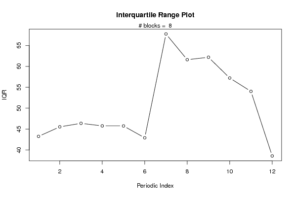
| Title produced by software | Standard Deviation Plot | ||||||||||||||||||||
| Date of computation | Sun, 16 Aug 2009 10:16:11 -0600 | ||||||||||||||||||||
| Cite this page as follows | Statistical Computations at FreeStatistics.org, Office for Research Development and Education, URL https://freestatistics.org/blog/index.php?v=date/2009/Aug/16/t12504394051vcdaa7k01zhzjv.htm/, Retrieved Sun, 05 May 2024 17:19:12 +0000 | ||||||||||||||||||||
| Statistical Computations at FreeStatistics.org, Office for Research Development and Education, URL https://freestatistics.org/blog/index.php?pk=42658, Retrieved Sun, 05 May 2024 17:19:12 +0000 | |||||||||||||||||||||
| QR Codes: | |||||||||||||||||||||
|
| |||||||||||||||||||||
| Original text written by user: | |||||||||||||||||||||
| IsPrivate? | No (this computation is public) | ||||||||||||||||||||
| User-defined keywords | |||||||||||||||||||||
| Estimated Impact | 163 | ||||||||||||||||||||
Tree of Dependent Computations | |||||||||||||||||||||
| Family? (F = Feedback message, R = changed R code, M = changed R Module, P = changed Parameters, D = changed Data) | |||||||||||||||||||||
| - [Central Tendency] [Maarten Verhaegen...] [2008-08-17 13:34:14] [b57209f6d0b19d479b8c06a8ae81c48a] - RMPD [Standard Deviation Plot] [] [2009-08-16 16:16:11] [e921d89db97faa9283224ee60d8fb091] [Current] | |||||||||||||||||||||
| Feedback Forum | |||||||||||||||||||||
Post a new message | |||||||||||||||||||||
Dataset | |||||||||||||||||||||
| Dataseries X: | |||||||||||||||||||||
72.84 73.96 73.26 73.86 73.04 212.8 157.92 111.55 99.01 89.5 100.95 116.06 131.5 137.43 138.53 137.26 136.81 182.98 149.45 109.34 93.37 84.09 83.83 82.94 82.88 81.41 79.87 79.66 76.07 182.69 165.78 142.5 120.6 105.73 98.72 98.41 96.08 97.3 97.5 97.02 98.75 232.81 240.83 193.4 148.28 138.34 135.34 134.02 133.86 131.67 132.43 130.21 129.98 206.16 195.17 159.16 136.33 125.18 121.21 119.38 119.26 119.75 118.78 116.97 121.69 223.51 228.58 205.22 189.4 180.14 177.59 176.39 171.16 173.11 171.74 175.97 179.64 254.62 240.5 212.01 176.36 153.24 146.69 141.52 142.6 143.19 142.32 142.03 144.92 177.31 194.4 189.19 180.44 175.84 178.54 176.55 | |||||||||||||||||||||
Tables (Output of Computation) | |||||||||||||||||||||
| |||||||||||||||||||||
Figures (Output of Computation) | |||||||||||||||||||||
Input Parameters & R Code | |||||||||||||||||||||
| Parameters (Session): | |||||||||||||||||||||
| par2 = grey ; par3 = FALSE ; par4 = Unknown ; | |||||||||||||||||||||
| Parameters (R input): | |||||||||||||||||||||
| par1 = 12 ; | |||||||||||||||||||||
| R code (references can be found in the software module): | |||||||||||||||||||||
par1 <- as.numeric(par1) | |||||||||||||||||||||