Free Statistics
of Irreproducible Research!
Description of Statistical Computation | |||||||||||||||||||||||||||||||||||||||||||||||||||||||||||||||||||||||||||||||||
|---|---|---|---|---|---|---|---|---|---|---|---|---|---|---|---|---|---|---|---|---|---|---|---|---|---|---|---|---|---|---|---|---|---|---|---|---|---|---|---|---|---|---|---|---|---|---|---|---|---|---|---|---|---|---|---|---|---|---|---|---|---|---|---|---|---|---|---|---|---|---|---|---|---|---|---|---|---|---|---|---|---|
| Author's title | |||||||||||||||||||||||||||||||||||||||||||||||||||||||||||||||||||||||||||||||||
| Author | *Unverified author* | ||||||||||||||||||||||||||||||||||||||||||||||||||||||||||||||||||||||||||||||||
| R Software Module | rwasp_bootstrapplot.wasp | ||||||||||||||||||||||||||||||||||||||||||||||||||||||||||||||||||||||||||||||||
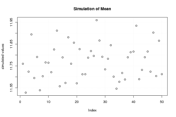
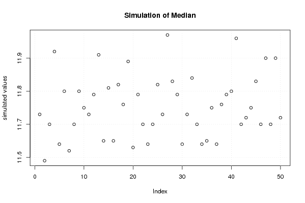
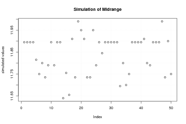
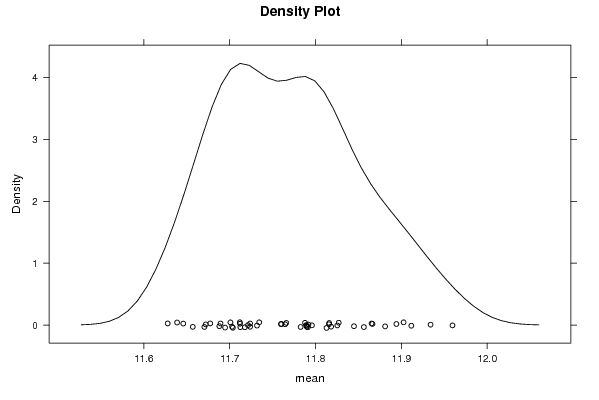
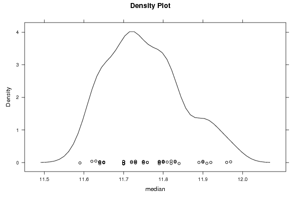
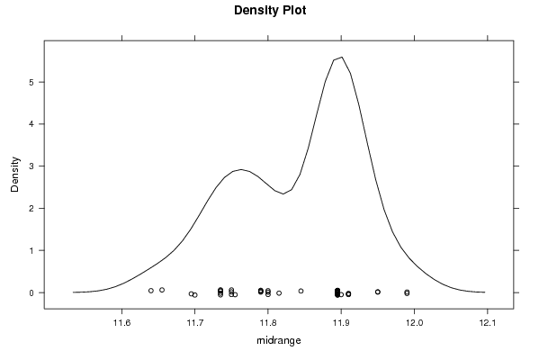
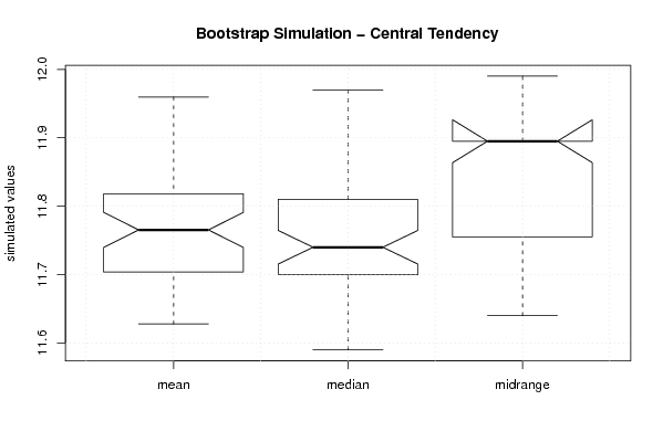
| Title produced by software | Blocked Bootstrap Plot - Central Tendency | ||||||||||||||||||||||||||||||||||||||||||||||||||||||||||||||||||||||||||||||||
| Date of computation | Wed, 05 Aug 2009 12:54:30 -0600 | ||||||||||||||||||||||||||||||||||||||||||||||||||||||||||||||||||||||||||||||||
| Cite this page as follows | Statistical Computations at FreeStatistics.org, Office for Research Development and Education, URL https://freestatistics.org/blog/index.php?v=date/2009/Aug/05/t1249498541rnq1nsq7hisowun.htm/, Retrieved Sun, 13 Jul 2025 12:02:02 +0000 | ||||||||||||||||||||||||||||||||||||||||||||||||||||||||||||||||||||||||||||||||
| Statistical Computations at FreeStatistics.org, Office for Research Development and Education, URL https://freestatistics.org/blog/index.php?pk=42503, Retrieved Sun, 13 Jul 2025 12:02:02 +0000 | |||||||||||||||||||||||||||||||||||||||||||||||||||||||||||||||||||||||||||||||||
| QR Codes: | |||||||||||||||||||||||||||||||||||||||||||||||||||||||||||||||||||||||||||||||||
|
| |||||||||||||||||||||||||||||||||||||||||||||||||||||||||||||||||||||||||||||||||
| Original text written by user: | |||||||||||||||||||||||||||||||||||||||||||||||||||||||||||||||||||||||||||||||||
| IsPrivate? | No (this computation is public) | ||||||||||||||||||||||||||||||||||||||||||||||||||||||||||||||||||||||||||||||||
| User-defined keywords | |||||||||||||||||||||||||||||||||||||||||||||||||||||||||||||||||||||||||||||||||
| Estimated Impact | 304 | ||||||||||||||||||||||||||||||||||||||||||||||||||||||||||||||||||||||||||||||||
Tree of Dependent Computations | |||||||||||||||||||||||||||||||||||||||||||||||||||||||||||||||||||||||||||||||||
| Family? (F = Feedback message, R = changed R code, M = changed R Module, P = changed Parameters, D = changed Data) | |||||||||||||||||||||||||||||||||||||||||||||||||||||||||||||||||||||||||||||||||
| - [Bootstrap Plot - Central Tendency] [Bootstrap plot ma...] [2009-08-05 15:54:55] [b61406873bd841e2047c054f7ebec102] - RMPD [Blocked Bootstrap Plot - Central Tendency] [Bootstrap plot ge...] [2009-08-05 18:54:30] [f78fa5e3827314a0edd0041d1d9dae5e] [Current] - RMPD [Variability] [Spreidingsmaten m...] [2009-08-06 10:01:18] [b61406873bd841e2047c054f7ebec102] - RMP [Variability] [Spreidingsmaten g...] [2009-08-06 10:09:49] [b61406873bd841e2047c054f7ebec102] - RMP [Standard Deviation Plot] [Standaarddeviatie...] [2009-08-06 11:24:11] [b61406873bd841e2047c054f7ebec102] - RMP [Standard Deviation-Mean Plot] [Standardeviation ...] [2009-08-06 12:17:08] [b61406873bd841e2047c054f7ebec102] - RMP [Classical Decomposition] [Classical decompo...] [2009-08-06 12:26:35] [b61406873bd841e2047c054f7ebec102] - RMP [Classical Decomposition] [Classical decompo...] [2009-08-06 12:26:35] [b61406873bd841e2047c054f7ebec102] - RMP [Classical Decomposition] [Classical decompo...] [2009-08-06 12:26:35] [b61406873bd841e2047c054f7ebec102] - RMP [Exponential Smoothing] [Exponential smoot...] [2009-08-06 22:31:35] [74be16979710d4c4e7c6647856088456] | |||||||||||||||||||||||||||||||||||||||||||||||||||||||||||||||||||||||||||||||||
| Feedback Forum | |||||||||||||||||||||||||||||||||||||||||||||||||||||||||||||||||||||||||||||||||
Post a new message | |||||||||||||||||||||||||||||||||||||||||||||||||||||||||||||||||||||||||||||||||
Dataset | |||||||||||||||||||||||||||||||||||||||||||||||||||||||||||||||||||||||||||||||||
| Dataseries X: | |||||||||||||||||||||||||||||||||||||||||||||||||||||||||||||||||||||||||||||||||
11,73 11,74 11,65 11,38 11,53 11,75 11,82 11,83 11,63 11,55 11,4 11,4 11,63 11,46 11,35 11,7 11,52 11,64 11,9 11,73 11,7 11,54 11,97 11,64 11,98 11,79 11,66 11,96 11,83 12,36 12,53 12,55 12,53 12,24 12,34 12,05 12,22 12,23 11,92 12,13 12,1 12,15 12,23 12,08 12,02 11,93 12,16 11,87 11,93 11,79 11,43 11,63 11,93 11,89 11,83 11,59 12,04 11,81 11,9 11,72 11,91 11,94 11,91 11,84 12,01 11,89 11,8 11,7 11,5 11,76 11,61 11,27 11,64 11,39 11,54 11,62 11,59 11,44 11,31 11,56 11,4 11,51 11,5 11,24 11,8 | |||||||||||||||||||||||||||||||||||||||||||||||||||||||||||||||||||||||||||||||||
Tables (Output of Computation) | |||||||||||||||||||||||||||||||||||||||||||||||||||||||||||||||||||||||||||||||||
| |||||||||||||||||||||||||||||||||||||||||||||||||||||||||||||||||||||||||||||||||
Figures (Output of Computation) | |||||||||||||||||||||||||||||||||||||||||||||||||||||||||||||||||||||||||||||||||
Input Parameters & R Code | |||||||||||||||||||||||||||||||||||||||||||||||||||||||||||||||||||||||||||||||||
| Parameters (Session): | |||||||||||||||||||||||||||||||||||||||||||||||||||||||||||||||||||||||||||||||||
| par1 = 50 ; par2 = 12 ; | |||||||||||||||||||||||||||||||||||||||||||||||||||||||||||||||||||||||||||||||||
| Parameters (R input): | |||||||||||||||||||||||||||||||||||||||||||||||||||||||||||||||||||||||||||||||||
| par1 = 50 ; par2 = 12 ; | |||||||||||||||||||||||||||||||||||||||||||||||||||||||||||||||||||||||||||||||||
| R code (references can be found in the software module): | |||||||||||||||||||||||||||||||||||||||||||||||||||||||||||||||||||||||||||||||||
par1 <- as.numeric(par1) | |||||||||||||||||||||||||||||||||||||||||||||||||||||||||||||||||||||||||||||||||