Free Statistics
of Irreproducible Research!
Description of Statistical Computation | |||||||||||||||||||||||||||||||||||||||
|---|---|---|---|---|---|---|---|---|---|---|---|---|---|---|---|---|---|---|---|---|---|---|---|---|---|---|---|---|---|---|---|---|---|---|---|---|---|---|---|
| Author's title | |||||||||||||||||||||||||||||||||||||||
| Author | *The author of this computation has been verified* | ||||||||||||||||||||||||||||||||||||||
| R Software Module | rwasp_fitdistrnorm.wasp | ||||||||||||||||||||||||||||||||||||||
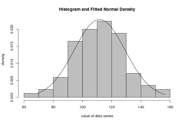
| Title produced by software | Maximum-likelihood Fitting - Normal Distribution | ||||||||||||||||||||||||||||||||||||||
| Date of computation | Wed, 12 Nov 2008 08:50:16 -0700 | ||||||||||||||||||||||||||||||||||||||
| Cite this page as follows | Statistical Computations at FreeStatistics.org, Office for Research Development and Education, URL https://freestatistics.org/blog/index.php?v=date/2008/Nov/12/t12265050590vkypsuifpmnqfe.htm/, Retrieved Sat, 05 Jul 2025 17:55:28 +0000 | ||||||||||||||||||||||||||||||||||||||
| Statistical Computations at FreeStatistics.org, Office for Research Development and Education, URL https://freestatistics.org/blog/index.php?pk=24255, Retrieved Sat, 05 Jul 2025 17:55:28 +0000 | |||||||||||||||||||||||||||||||||||||||
| QR Codes: | |||||||||||||||||||||||||||||||||||||||
|
| |||||||||||||||||||||||||||||||||||||||
| Original text written by user: | |||||||||||||||||||||||||||||||||||||||
| IsPrivate? | No (this computation is public) | ||||||||||||||||||||||||||||||||||||||
| User-defined keywords | |||||||||||||||||||||||||||||||||||||||
| Estimated Impact | 230 | ||||||||||||||||||||||||||||||||||||||
Tree of Dependent Computations | |||||||||||||||||||||||||||||||||||||||
| Family? (F = Feedback message, R = changed R code, M = changed R Module, P = changed Parameters, D = changed Data) | |||||||||||||||||||||||||||||||||||||||
| F [Maximum-likelihood Fitting - Normal Distribution] [Various EDA Topics ] [2008-11-12 15:50:16] [e7b1048c2c3a353441b9143db4404b91] [Current] - D [Maximum-likelihood Fitting - Normal Distribution] [Paper maximum lik...] [2008-12-19 17:54:18] [1640119c345fbfa2091dc1243f79f7a6] | |||||||||||||||||||||||||||||||||||||||
| Feedback Forum | |||||||||||||||||||||||||||||||||||||||
Post a new message | |||||||||||||||||||||||||||||||||||||||
Dataset | |||||||||||||||||||||||||||||||||||||||
| Dataseries X: | |||||||||||||||||||||||||||||||||||||||
78,4 114,6 113,3 117,0 99,6 99,4 101,9 115,2 108,5 113,8 121,0 92,2 90,2 101,5 126,6 93,9 89,8 93,4 101,5 110,4 105,9 108,4 113,9 86,1 69,4 101,2 100,5 98,0 106,6 90,1 96,9 125,9 112,0 100,0 123,9 79,8 83,4 113,6 112,9 104,0 109,9 99,0 106,3 128,9 111,1 102,9 130,0 87,0 87,5 117,6 103,4 110,8 112,6 102,5 112,4 135,6 105,1 127,7 137,0 91,0 90,5 122,4 123,3 124,3 120,0 118,1 119,0 142,7 123,6 129,6 151,6 110,4 99,2 130,5 136,2 129,7 128,0 121,6 135,8 143,8 147,5 136,2 156,6 123,3 100,4 | |||||||||||||||||||||||||||||||||||||||
Tables (Output of Computation) | |||||||||||||||||||||||||||||||||||||||
| |||||||||||||||||||||||||||||||||||||||
Figures (Output of Computation) | |||||||||||||||||||||||||||||||||||||||
Input Parameters & R Code | |||||||||||||||||||||||||||||||||||||||
| Parameters (Session): | |||||||||||||||||||||||||||||||||||||||
| par1 = 8 ; par2 = 0 ; | |||||||||||||||||||||||||||||||||||||||
| Parameters (R input): | |||||||||||||||||||||||||||||||||||||||
| par1 = 8 ; par2 = 0 ; | |||||||||||||||||||||||||||||||||||||||
| R code (references can be found in the software module): | |||||||||||||||||||||||||||||||||||||||
library(MASS) | |||||||||||||||||||||||||||||||||||||||