Repository of Reproducible Computations

Free Statistics

of Irreproducible Research!

Author's title

Author

*The author of this computation has been verified*

R Software Module

rwasp_boxcoxlin.wasp

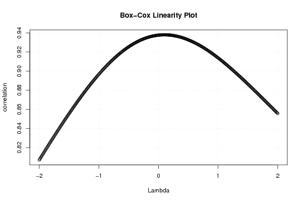
Title produced by software

Box-Cox Linearity Plot

Date of computation

Tue, 11 Nov 2008 12:49:52 -0700

Cite this page as follows

Statistical Computations at FreeStatistics.org, Office for Research Development and Education, URL https://freestatistics.org/blog/index.php?v=date/2008/Nov/11/t1226433073jg9b5n9lh73313c.htm/, Retrieved Mon, 20 May 2024 11:17:52 +0000

Statistical Computations at FreeStatistics.org, Office for Research Development and Education, URL https://freestatistics.org/blog/index.php?pk=23904, Retrieved Mon, 20 May 2024 11:17:52 +0000

QR Codes:

Paste this QR Code to cite your computation.

Original text written by user:

IsPrivate?

No (this computation is public)

User-defined keywords

Bert Moons

Estimated Impact

126

Family? (F = Feedback message, R = changed R code, M = changed R Module, P = changed Parameters, D = changed Data)

-     [Box-Cox Linearity Plot] [Bert Moons - Q3 B...] [2008-11-11 10:17:28] [b6c777429d07a05453509ef079833861]
F R  D    [Box-Cox Linearity Plot] [Bert Moons - Box-...] [2008-11-11 19:49:52] [1828943283e41f5e3270e2e73d6433b4] [Current]

Feedback Forum

2008-11-19 17:50:13 [Toon Wouters] [reply] 
Het is een min of meer juiste conclusie die je maakt. De box-cox linearity plot word bekomen door de scatterplot te transformeren en lieaire te maken. En dan hopen dat de curve een maximum toont en dit is inderdaad het geval bij lambda = 0 en kun je concluderen dat 0 de optimale correlatie is
2008-11-20 15:33:56 [Natalie De Wilde] [reply] 
Wanneer er een parabool met een maximum wordt bereikt, dan heb je de beste transformatie gedaan.Zoals je zegt is de optimale transformatie gevonden bij lambda 0,1. 
Er is een klein verschil na de transformatie van de Linear Fit of original data, de punten onder de lijn zijn naar boven opgeschoven.
2008-11-24 18:42:11 [Sören Van Donink] [reply] 
Een optimale transformatie  zou moeten leiden tot een bergparabool wat ook het geval is. De optimale transformatie kan inderdaad gevonden worden bij lambda 0,1 . 
Er is inderdaad een miniem verschil na het doorvoeren van de transformatie van de Linear Fit.
2008-11-24 20:43:35 [Vincent Vanden Poel] [reply] 
een Box Cox Line brengt 2 variabelen met elkaar in verband. Het is een stijgende of dalende lijn. Men laat de X varieren van -2 tot +2 en gaat vervolgens de correlatie berekenen tussen Y en de getransformeerde X. Aan de hand van de transformatie van X wil men alle punten op een lineaire rechte krijgen. Een MAX waarde is de ideale waarde om het scatterplot te linealiseren. In dit geval is dit inderdaad 0,1 (+/- 0). Maar zoals je zelf hebt aangegeven is de lineaire overeenkomst nauwelijks verbeterd na de transformatie.

Post a new message

Dataseries X:

Download CSV

Histogram

Boxplots

4,8
5,5
5,4
5,9
5,8
5,1
4,1
4,4
3,6
3,5
3,1
2,9
2,2
1,4
1,2
1,3
1,3
1,3
1,8
1,8
1,8
1,7
2,1
2
1,7
1,9
2,3
2,4
2,5
2,8
2,6
2,2
2,8
2,8
2,8
2,3
2,2
3
2,9
2,7
2,7
2,3
2,4
2,8
2,3
2
1,9
2,3
2,7
1,8
2
2,1
2
2,4
1,7
1
1,2
1,4
1,7
1,8

Dataseries Y:

Download CSV

Histogram

19,2
26,6
26,6
31,4
31,2
26,4
20,7
20,7
15
13,3
8,7
10,2
4,3
-0,1
-4,6
-3,9
-3,5
-3,4
-2,5
-1,1
0,3
-0,9
3,6
2,7
-0,2
-1
5,8
6,4
9,6
13,2
10,6
10,9
12,9
15,9
12,2
9,1
9
17,4
14,7
17
13,7
9,5
14,8
13,6
12,6
8,9
10,2
12,7
16
10,4
9,9
9,5
8,6
10
3,5
-4,2
-4,4
-1,5
-0,1
0,8

Summary of computational transaction
Raw Input	view raw input (R code)
Raw Output	view raw output of R engine
Computing time	2 seconds
R Server	'Sir Ronald Aylmer Fisher' @ 193.190.124.24

\begin{tabular}{lllllllll}
\hline
Summary of computational transaction \tabularnewline
Raw Input & view raw input (R code)  \tabularnewline
Raw Output & view raw output of R engine  \tabularnewline
Computing time & 2 seconds \tabularnewline
R Server & 'Sir Ronald Aylmer Fisher' @ 193.190.124.24 \tabularnewline
\hline
\end{tabular}
%Source: https://freestatistics.org/blog/index.php?pk=23904&T=0

[TABLE]
[ROW][C]Summary of computational transaction[/C][/ROW]
[ROW][C]Raw Input[/C][C]view raw input (R code) [/C][/ROW]
[ROW][C]Raw Output[/C][C]view raw output of R engine [/C][/ROW]
[ROW][C]Computing time[/C][C]2 seconds[/C][/ROW]
[ROW][C]R Server[/C][C]'Sir Ronald Aylmer Fisher' @ 193.190.124.24[/C][/ROW]
[/TABLE]
Source: https://freestatistics.org/blog/index.php?pk=23904&T=0

Globally Unique Identifier (entire table): ba.freestatistics.org/blog/index.php?pk=23904&T=0

As an alternative you can also use a QR Code:

The GUIDs for individual cells are displayed in the table below:

Summary of computational transaction
Raw Input	view raw input (R code)
Raw Output	view raw output of R engine
Computing time	2 seconds
R Server	'Sir Ronald Aylmer Fisher' @ 193.190.124.24

Box-Cox Linearity Plot
# observations x	60
maximum correlation	0.93797935752351
optimal lambda(x)	0.1
Residual SD (orginial)	3.68425145440835
Residual SD (transformed)	3.14543649064313

\begin{tabular}{lllllllll}
\hline
Box-Cox Linearity Plot \tabularnewline
# observations x & 60 \tabularnewline
maximum correlation & 0.93797935752351 \tabularnewline
optimal lambda(x) & 0.1 \tabularnewline
Residual SD (orginial) & 3.68425145440835 \tabularnewline
Residual SD (transformed) & 3.14543649064313 \tabularnewline
\hline
\end{tabular}
%Source: https://freestatistics.org/blog/index.php?pk=23904&T=1

[TABLE]
[ROW][C]Box-Cox Linearity Plot[/C][/ROW]
[ROW][C]# observations x[/C][C]60[/C][/ROW]
[ROW][C]maximum correlation[/C][C]0.93797935752351[/C][/ROW]
[ROW][C]optimal lambda(x)[/C][C]0.1[/C][/ROW]
[ROW][C]Residual SD (orginial)[/C][C]3.68425145440835[/C][/ROW]
[ROW][C]Residual SD (transformed)[/C][C]3.14543649064313[/C][/ROW]
[/TABLE]
Source: https://freestatistics.org/blog/index.php?pk=23904&T=1

Globally Unique Identifier (entire table): ba.freestatistics.org/blog/index.php?pk=23904&T=1

As an alternative you can also use a QR Code:

The GUIDs for individual cells are displayed in the table below:

Box-Cox Linearity Plot
# observations x	60
maximum correlation	0.93797935752351
optimal lambda(x)	0.1
Residual SD (orginial)	3.68425145440835
Residual SD (transformed)	3.14543649064313

Figure 1

PNG link

Postscript link

PDF link

Figure 2

PNG link

Postscript link

PDF link

Figure 3

PNG link

Postscript link

PDF link

Parameters (Session):

Parameters (R input):

R code (references can be found in the software module):

n <- length(x)
c <- array(NA,dim=c(401))
l <- array(NA,dim=c(401))
mx <- 0
mxli <- -999
for (i in 1:401)
{
l[i] <- (i-201)/100
if (l[i] != 0)
{
x1 <- (x^l[i] - 1) / l[i]
} else {
x1 <- log(x)
}
c[i] <- cor(x1,y)
if (mx < abs(c[i]))
{
mx <- abs(c[i])
mxli <- l[i]
}
}
c
mx
mxli
if (mxli != 0)
{
x1 <- (x^mxli - 1) / mxli
} else {
x1 <- log(x)
}
r<-lm(y~x)
se <- sqrt(var(r$residuals))
r1 <- lm(y~x1)
se1 <- sqrt(var(r1$residuals))
bitmap(file='test1.png')
plot(l,c,main='Box-Cox Linearity Plot',xlab='Lambda',ylab='correlation')
grid()
dev.off()
bitmap(file='test2.png')
plot(x,y,main='Linear Fit of Original Data',xlab='x',ylab='y')
abline(r)
grid()
mtext(paste('Residual Standard Deviation = ',se))
dev.off()
bitmap(file='test3.png')
plot(x1,y,main='Linear Fit of Transformed Data',xlab='x',ylab='y')
abline(r1)
grid()
mtext(paste('Residual Standard Deviation = ',se1))
dev.off()
load(file='createtable')
a<-table.start()
a<-table.row.start(a)
a<-table.element(a,'Box-Cox Linearity Plot',2,TRUE)
a<-table.row.end(a)
a<-table.row.start(a)
a<-table.element(a,'# observations x',header=TRUE)
a<-table.element(a,n)
a<-table.row.end(a)
a<-table.row.start(a)
a<-table.element(a,'maximum correlation',header=TRUE)
a<-table.element(a,mx)
a<-table.row.end(a)
a<-table.row.start(a)
a<-table.element(a,'optimal lambda(x)',header=TRUE)
a<-table.element(a,mxli)
a<-table.row.end(a)
a<-table.row.start(a)
a<-table.element(a,'Residual SD (orginial)',header=TRUE)
a<-table.element(a,se)
a<-table.row.end(a)
a<-table.row.start(a)
a<-table.element(a,'Residual SD (transformed)',header=TRUE)
a<-table.element(a,se1)
a<-table.row.end(a)
a<-table.end(a)
table.save(a,file='mytable.tab')

Free Statistics

Description of Statistical Computation

Tree of Dependent Computations

Dataset

Tables (Output of Computation)

Figures (Output of Computation)

Input Parameters & R Code