Free Statistics
of Irreproducible Research!
Description of Statistical Computation | |||||||||||||||||||||
|---|---|---|---|---|---|---|---|---|---|---|---|---|---|---|---|---|---|---|---|---|---|
| Author's title | |||||||||||||||||||||
| Author | *The author of this computation has been verified* | ||||||||||||||||||||
| R Software Module | rwasp_cloud.wasp | ||||||||||||||||||||
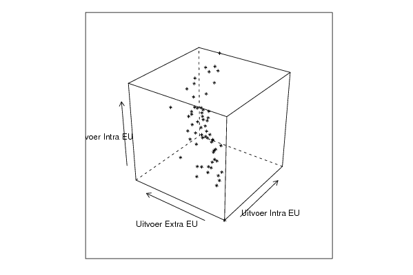
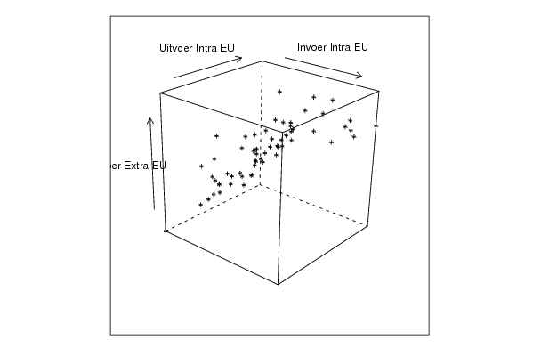
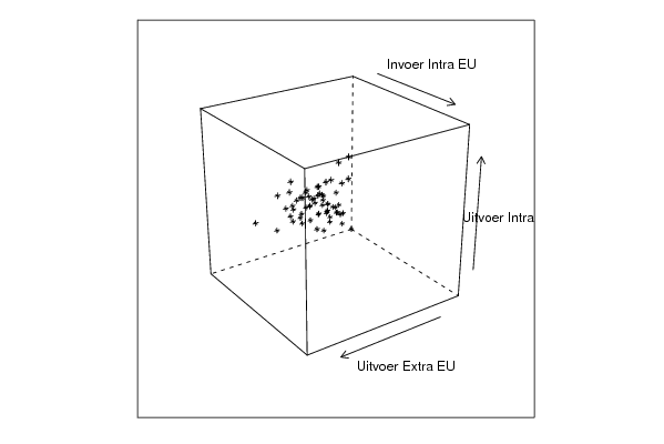
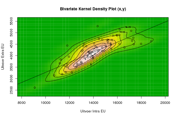
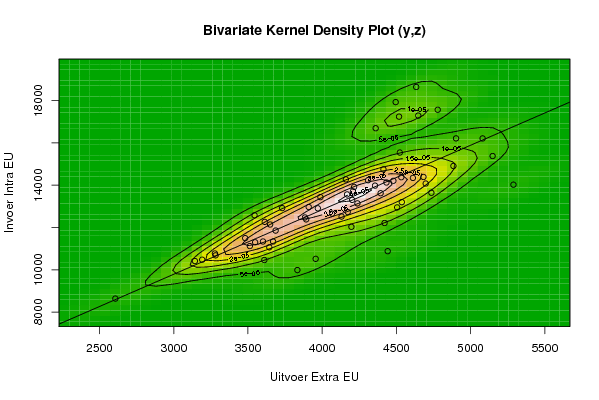
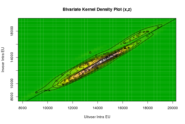
| Title produced by software | Trivariate Scatterplots | ||||||||||||||||||||
| Date of computation | Tue, 11 Nov 2008 08:58:30 -0700 | ||||||||||||||||||||
| Cite this page as follows | Statistical Computations at FreeStatistics.org, Office for Research Development and Education, URL https://freestatistics.org/blog/index.php?v=date/2008/Nov/11/t1226419226wp219i7ed6fbfzd.htm/, Retrieved Sat, 12 Jul 2025 10:04:43 +0000 | ||||||||||||||||||||
| Statistical Computations at FreeStatistics.org, Office for Research Development and Education, URL https://freestatistics.org/blog/index.php?pk=23623, Retrieved Sat, 12 Jul 2025 10:04:43 +0000 | |||||||||||||||||||||
| QR Codes: | |||||||||||||||||||||
|
| |||||||||||||||||||||
| Original text written by user: | |||||||||||||||||||||
| IsPrivate? | No (this computation is public) | ||||||||||||||||||||
| User-defined keywords | |||||||||||||||||||||
| Estimated Impact | 222 | ||||||||||||||||||||
Tree of Dependent Computations | |||||||||||||||||||||
| Family? (F = Feedback message, R = changed R code, M = changed R Module, P = changed Parameters, D = changed Data) | |||||||||||||||||||||
| F [Exercise 1.13] [Exercise 1.13 (Wo...] [2008-10-01 13:28:34] [b98453cac15ba1066b407e146608df68] - RMPD [Univariate Data Series] [Time series 1] [2008-10-13 19:38:20] [7496c02ff89a4d46194b78685600e356] F RMPD [Bivariate Kernel Density Estimation] [Q1] [2008-11-11 15:51:32] [299afd6311e4c20059ea2f05c8dd029d] - RMPD [Trivariate Scatterplots] [Q1 Trivariate Sca...] [2008-11-11 15:58:30] [5e2b1e7aa808f9f0d23fd35605d4968f] [Current] | |||||||||||||||||||||
| Feedback Forum | |||||||||||||||||||||
Post a new message | |||||||||||||||||||||
Dataset | |||||||||||||||||||||
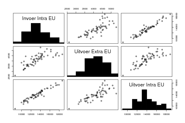
| Dataseries X: | |||||||||||||||||||||
12192.5 11268.8 9097.4 12639.8 13040.1 11687.3 11191.7 11391.9 11793.1 13933.2 12778.1 11810.3 13698.4 11956.6 10723.8 13938.9 13979.8 13807.4 12973.9 12509.8 12934.1 14908.3 13772.1 13012.6 14049.9 11816.5 11593.2 14466.2 13615.9 14733.9 13880.7 13527.5 13584 16170.2 13260.6 14741.9 15486.5 13154.5 12621.2 15031.6 15452.4 15428 13105.9 14716.8 14180 16202.2 14392.4 15140.6 15960.1 14351.3 13230.2 15202.1 17157.3 16159.1 13405.7 17224.7 17338.4 17370.6 18817.8 16593.2 17979.5 | |||||||||||||||||||||
| Dataseries Y: | |||||||||||||||||||||
3277.2 3833 2606.3 3643.8 3686.4 3281.6 3669.3 3191.5 3512.7 3970.7 3601.2 3610 4172.1 3956.2 3142.7 3884.3 3892.2 3613 3730.5 3481.3 3649.5 4215.2 4066.6 4196.8 4536.6 4441.6 3548.3 4735.9 4130.6 4356.2 4159.6 3988 4167.8 4902.2 3909.4 4697.6 4308.9 4420.4 3544.2 4433 4479.7 4533.2 4237.5 4207.4 4394 5148.4 4202.2 4682.5 4884.3 5288.9 4505.2 4611.5 5081.1 4523.1 4412.8 4647.4 4778.6 4495.3 4633.5 4360.5 4517.9 | |||||||||||||||||||||
| Dataseries Z: | |||||||||||||||||||||
10772.8 9987.7 8638.7 11063.7 11855.7 10684.5 11337.4 10478 11123.9 12909.3 11339.9 10462.2 12733.5 10519.2 10414.9 12476.8 12384.6 12266.7 12919.9 11497.3 12142 13919.4 12656.8 12034.1 13199.7 10881.3 11301.2 13643.9 12517 13981.1 14275.7 13435 13565.7 16216.3 12970 14079.9 14235 12213.4 12581 14130.4 14210.8 14378.5 13142.8 13714.7 13621.9 15379.8 13306.3 14391.2 14909.9 14025.4 12951.2 14344.3 16213.3 15544.5 14750.6 17292.7 17568.5 17930.8 18644.7 16694.8 17242.8 | |||||||||||||||||||||
Tables (Output of Computation) | |||||||||||||||||||||
| |||||||||||||||||||||
Figures (Output of Computation) | |||||||||||||||||||||
Input Parameters & R Code | |||||||||||||||||||||
| Parameters (Session): | |||||||||||||||||||||
| par1 = 50 ; par2 = 50 ; par3 = Y ; par4 = Y ; par5 = Uitvoer Intra EU ; par6 = Uitvoer Extra EU ; par7 = Invoer Intra EU ; | |||||||||||||||||||||
| Parameters (R input): | |||||||||||||||||||||
| par1 = 50 ; par2 = 50 ; par3 = Y ; par4 = Y ; par5 = Uitvoer Intra EU ; par6 = Uitvoer Extra EU ; par7 = Invoer Intra EU ; | |||||||||||||||||||||
| R code (references can be found in the software module): | |||||||||||||||||||||
x <- array(x,dim=c(length(x),1)) | |||||||||||||||||||||