\begin{tabular}{lllllllll}
\hline
Summary of compuational transaction \tabularnewline
Raw Input & view raw input (R code)  \tabularnewline
Raw Output & view raw output of R engine  \tabularnewline
Computing time & 1 seconds \tabularnewline
R Server & 'George Udny Yule' @ 72.249.76.132 \tabularnewline
\hline
\end{tabular}
%Source: https://freestatistics.org/blog/index.php?pk=8021&T=0
[TABLE]
[ROW][C]Summary of compuational transaction[/C][/ROW]
[ROW][C]Raw Input[/C][C]view raw input (R code) [/C][/ROW]
[ROW][C]Raw Output[/C][C]view raw output of R engine [/C][/ROW]
[ROW][C]Computing time[/C][C]1 seconds[/C][/ROW]
[ROW][C]R Server[/C][C]'George Udny Yule' @ 72.249.76.132[/C][/ROW]
[/TABLE]
Source: https://freestatistics.org/blog/index.php?pk=8021&T=0
If you paste this QR Code into your document, anyone with a smartphone or tablet will be able to scan it and view this table in a browser.
If you paste this QR Code into your document, anyone with a smartphone or tablet will be able to scan it and view this table in a browser.
If you paste this QR Code into your document, anyone with a smartphone or tablet will be able to scan it and view this table in a browser.
If you paste this QR Code into your document, anyone with a smartphone or tablet will be able to scan it and view this table in a browser.
If you paste this QR Code into your document, anyone with a smartphone or tablet will be able to scan it and view this table in a browser.
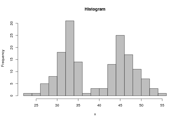
| Frequency Table (Histogram) | | Bins | Midpoint | Abs. Frequency | Rel. Frequency | Cumul. Rel. Freq. | Density | | [22,24[ | 23 | 1 | 0.006173 | 0.006173 | 0.003086 | | [24,26[ | 25 | 1 | 0.006173 | 0.012346 | 0.003086 | | [26,28[ | 27 | 5 | 0.030864 | 0.04321 | 0.015432 | | [28,30[ | 29 | 8 | 0.049383 | 0.092593 | 0.024691 | | [30,32[ | 31 | 18 | 0.111111 | 0.203704 | 0.055556 | | [32,34[ | 33 | 31 | 0.191358 | 0.395062 | 0.095679 | | [34,36[ | 35 | 14 | 0.08642 | 0.481481 | 0.04321 | | [36,38[ | 37 | 1 | 0.006173 | 0.487654 | 0.003086 | | [38,40[ | 39 | 3 | 0.018519 | 0.506173 | 0.009259 | | [40,42[ | 41 | 3 | 0.018519 | 0.524691 | 0.009259 | | [42,44[ | 43 | 13 | 0.080247 | 0.604938 | 0.040123 | | [44,46[ | 45 | 25 | 0.154321 | 0.759259 | 0.07716 | | [46,48[ | 47 | 17 | 0.104938 | 0.864198 | 0.052469 | | [48,50[ | 49 | 11 | 0.067901 | 0.932099 | 0.033951 | | [50,52[ | 51 | 7 | 0.04321 | 0.975309 | 0.021605 | | [52,54[ | 53 | 3 | 0.018519 | 0.993827 | 0.009259 | | [54,56[ | 55 | 1 | 0.006173 | 1 | 0.003086 |
\begin{tabular}{lllllllll}
\hline
Frequency Table (Histogram) \tabularnewline
Bins & Midpoint & Abs. Frequency & Rel. Frequency & Cumul. Rel. Freq. & Density \tabularnewline
[22,24[ & 23 & 1 & 0.006173 & 0.006173 & 0.003086 \tabularnewline
[24,26[ & 25 & 1 & 0.006173 & 0.012346 & 0.003086 \tabularnewline
[26,28[ & 27 & 5 & 0.030864 & 0.04321 & 0.015432 \tabularnewline
[28,30[ & 29 & 8 & 0.049383 & 0.092593 & 0.024691 \tabularnewline
[30,32[ & 31 & 18 & 0.111111 & 0.203704 & 0.055556 \tabularnewline
[32,34[ & 33 & 31 & 0.191358 & 0.395062 & 0.095679 \tabularnewline
[34,36[ & 35 & 14 & 0.08642 & 0.481481 & 0.04321 \tabularnewline
[36,38[ & 37 & 1 & 0.006173 & 0.487654 & 0.003086 \tabularnewline
[38,40[ & 39 & 3 & 0.018519 & 0.506173 & 0.009259 \tabularnewline
[40,42[ & 41 & 3 & 0.018519 & 0.524691 & 0.009259 \tabularnewline
[42,44[ & 43 & 13 & 0.080247 & 0.604938 & 0.040123 \tabularnewline
[44,46[ & 45 & 25 & 0.154321 & 0.759259 & 0.07716 \tabularnewline
[46,48[ & 47 & 17 & 0.104938 & 0.864198 & 0.052469 \tabularnewline
[48,50[ & 49 & 11 & 0.067901 & 0.932099 & 0.033951 \tabularnewline
[50,52[ & 51 & 7 & 0.04321 & 0.975309 & 0.021605 \tabularnewline
[52,54[ & 53 & 3 & 0.018519 & 0.993827 & 0.009259 \tabularnewline
[54,56[ & 55 & 1 & 0.006173 & 1 & 0.003086 \tabularnewline
\hline
\end{tabular}
%Source: https://freestatistics.org/blog/index.php?pk=8021&T=1
[TABLE]
[ROW][C]Frequency Table (Histogram)[/C][/ROW]
[ROW][C]Bins[/C][C]Midpoint[/C][C]Abs. Frequency[/C][C]Rel. Frequency[/C][C]Cumul. Rel. Freq.[/C][C]Density[/C][/ROW]
[ROW][C][22,24[[/C][C]23[/C][C]1[/C][C]0.006173[/C][C]0.006173[/C][C]0.003086[/C][/ROW]
[ROW][C][24,26[[/C][C]25[/C][C]1[/C][C]0.006173[/C][C]0.012346[/C][C]0.003086[/C][/ROW]
[ROW][C][26,28[[/C][C]27[/C][C]5[/C][C]0.030864[/C][C]0.04321[/C][C]0.015432[/C][/ROW]
[ROW][C][28,30[[/C][C]29[/C][C]8[/C][C]0.049383[/C][C]0.092593[/C][C]0.024691[/C][/ROW]
[ROW][C][30,32[[/C][C]31[/C][C]18[/C][C]0.111111[/C][C]0.203704[/C][C]0.055556[/C][/ROW]
[ROW][C][32,34[[/C][C]33[/C][C]31[/C][C]0.191358[/C][C]0.395062[/C][C]0.095679[/C][/ROW]
[ROW][C][34,36[[/C][C]35[/C][C]14[/C][C]0.08642[/C][C]0.481481[/C][C]0.04321[/C][/ROW]
[ROW][C][36,38[[/C][C]37[/C][C]1[/C][C]0.006173[/C][C]0.487654[/C][C]0.003086[/C][/ROW]
[ROW][C][38,40[[/C][C]39[/C][C]3[/C][C]0.018519[/C][C]0.506173[/C][C]0.009259[/C][/ROW]
[ROW][C][40,42[[/C][C]41[/C][C]3[/C][C]0.018519[/C][C]0.524691[/C][C]0.009259[/C][/ROW]
[ROW][C][42,44[[/C][C]43[/C][C]13[/C][C]0.080247[/C][C]0.604938[/C][C]0.040123[/C][/ROW]
[ROW][C][44,46[[/C][C]45[/C][C]25[/C][C]0.154321[/C][C]0.759259[/C][C]0.07716[/C][/ROW]
[ROW][C][46,48[[/C][C]47[/C][C]17[/C][C]0.104938[/C][C]0.864198[/C][C]0.052469[/C][/ROW]
[ROW][C][48,50[[/C][C]49[/C][C]11[/C][C]0.067901[/C][C]0.932099[/C][C]0.033951[/C][/ROW]
[ROW][C][50,52[[/C][C]51[/C][C]7[/C][C]0.04321[/C][C]0.975309[/C][C]0.021605[/C][/ROW]
[ROW][C][52,54[[/C][C]53[/C][C]3[/C][C]0.018519[/C][C]0.993827[/C][C]0.009259[/C][/ROW]
[ROW][C][54,56[[/C][C]55[/C][C]1[/C][C]0.006173[/C][C]1[/C][C]0.003086[/C][/ROW]
[/TABLE]
Source: https://freestatistics.org/blog/index.php?pk=8021&T=1
Globally Unique Identifier (entire table): ba.freestatistics.org/blog/index.php?pk=8021&T=1
As an alternative you can also use a QR Code:
The GUIDs for individual cells are displayed in the table below:
| Frequency Table (Histogram) | | Bins | Midpoint | Abs. Frequency | Rel. Frequency | Cumul. Rel. Freq. | Density | | [22,24[ | 23 | 1 | 0.006173 | 0.006173 | 0.003086 | | [24,26[ | 25 | 1 | 0.006173 | 0.012346 | 0.003086 | | [26,28[ | 27 | 5 | 0.030864 | 0.04321 | 0.015432 | | [28,30[ | 29 | 8 | 0.049383 | 0.092593 | 0.024691 | | [30,32[ | 31 | 18 | 0.111111 | 0.203704 | 0.055556 | | [32,34[ | 33 | 31 | 0.191358 | 0.395062 | 0.095679 | | [34,36[ | 35 | 14 | 0.08642 | 0.481481 | 0.04321 | | [36,38[ | 37 | 1 | 0.006173 | 0.487654 | 0.003086 | | [38,40[ | 39 | 3 | 0.018519 | 0.506173 | 0.009259 | | [40,42[ | 41 | 3 | 0.018519 | 0.524691 | 0.009259 | | [42,44[ | 43 | 13 | 0.080247 | 0.604938 | 0.040123 | | [44,46[ | 45 | 25 | 0.154321 | 0.759259 | 0.07716 | | [46,48[ | 47 | 17 | 0.104938 | 0.864198 | 0.052469 | | [48,50[ | 49 | 11 | 0.067901 | 0.932099 | 0.033951 | | [50,52[ | 51 | 7 | 0.04321 | 0.975309 | 0.021605 | | [52,54[ | 53 | 3 | 0.018519 | 0.993827 | 0.009259 | | [54,56[ | 55 | 1 | 0.006173 | 1 | 0.003086 |
If you paste this QR Code into your document, anyone with a smartphone or tablet will be able to scan it and view this table in a browser.
If you paste this QR Code into your document, anyone with a smartphone or tablet will be able to scan it and view this table in a browser.
If you paste this QR Code into your document, anyone with a smartphone or tablet will be able to scan it and view this table in a browser.
If you paste this QR Code into your document, anyone with a smartphone or tablet will be able to scan it and view this table in a browser.
If you paste this QR Code into your document, anyone with a smartphone or tablet will be able to scan it and view this table in a browser.
|