Repository of Reproducible Computations

Free Statistics

of Irreproducible Research!

Author's title

Author

*Unverified author*

R Software Module

rwasp_arimaforecasting.wasp

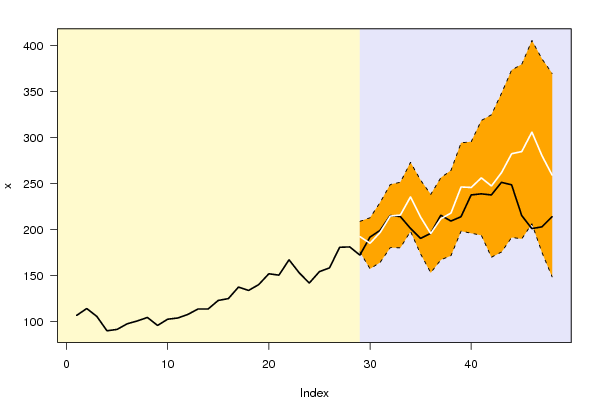
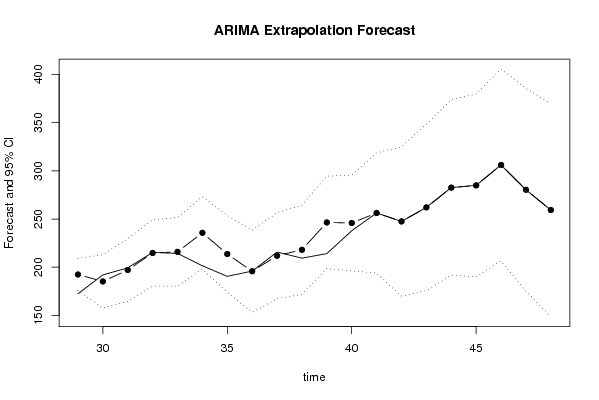
Title produced by software

ARIMA Forecasting

Date of computation

Mon, 07 Jan 2008 13:32:36 -0700

Cite this page as follows

Statistical Computations at FreeStatistics.org, Office for Research Development and Education, URL https://freestatistics.org/blog/index.php?v=date/2008/Jan/07/t1199737879ye2jtsfpk2dm3vv.htm/, Retrieved Mon, 06 May 2024 23:10:01 +0000

Statistical Computations at FreeStatistics.org, Office for Research Development and Education, URL https://freestatistics.org/blog/index.php?pk=7925, Retrieved Mon, 06 May 2024 23:10:01 +0000

QR Codes:

Paste this QR Code to cite your computation.

Original text written by user:

IsPrivate?

No (this computation is public)

User-defined keywords

Estimated Impact

303

Family? (F = Feedback message, R = changed R code, M = changed R Module, P = changed Parameters, D = changed Data)

-     [ARIMA Backward Selection] [ARMA backward sel...] [2007-12-20 15:28:14] [74be16979710d4c4e7c6647856088456]
- RMPD    [ARIMA Forecasting] [] [2008-01-07 20:32:36] [d41d8cd98f00b204e9800998ecf8427e] [Current]
-   PD      [ARIMA Forecasting] [werkloosheid/invoer] [2008-12-17 23:06:44] [5e74953d94072114d25d7276793b561e] 
-   P         [ARIMA Forecasting] [werkloosheid/invoer] [2008-12-19 10:13:06] [5e74953d94072114d25d7276793b561e] 
-   PD      [ARIMA Forecasting] [werkloosheid/invoer] [2008-12-17 23:09:12] [5e74953d94072114d25d7276793b561e] 
- RMPD      [Notched Boxplots] [de productie] [2008-12-17 23:17:54] [5e74953d94072114d25d7276793b561e] 
- RMPD      [Multiple Regression] [verband tussen in...] [2008-12-17 23:33:00] [5e74953d94072114d25d7276793b561e] 
- RMPD      [Multiple Regression] [verband tussen in...] [2008-12-17 23:36:56] [5e74953d94072114d25d7276793b561e] 
- RMPD      [Multiple Regression] [verband tussen in...] [2008-12-17 23:40:07] [5e74953d94072114d25d7276793b561e] 

Feedback Forum

Post a new message

Dataseries X:

Download CSV

Histogram

Boxplots

Summary of compuational transaction
Raw Input	view raw input (R code)
Raw Output	view raw output of R engine
Computing time	2 seconds
R Server	'Gwilym Jenkins' @ 72.249.127.135

\begin{tabular}{lllllllll}
\hline
Summary of compuational transaction \tabularnewline
Raw Input & view raw input (R code)  \tabularnewline
Raw Output & view raw output of R engine  \tabularnewline
Computing time & 2 seconds \tabularnewline
R Server & 'Gwilym Jenkins' @ 72.249.127.135 \tabularnewline
\hline
\end{tabular}
%Source: https://freestatistics.org/blog/index.php?pk=7925&T=0

[TABLE]
[ROW][C]Summary of compuational transaction[/C][/ROW]
[ROW][C]Raw Input[/C][C]view raw input (R code) [/C][/ROW]
[ROW][C]Raw Output[/C][C]view raw output of R engine [/C][/ROW]
[ROW][C]Computing time[/C][C]2 seconds[/C][/ROW]
[ROW][C]R Server[/C][C]'Gwilym Jenkins' @ 72.249.127.135[/C][/ROW]
[/TABLE]
Source: https://freestatistics.org/blog/index.php?pk=7925&T=0

Globally Unique Identifier (entire table): ba.freestatistics.org/blog/index.php?pk=7925&T=0

As an alternative you can also use a QR Code:

The GUIDs for individual cells are displayed in the table below:

Summary of compuational transaction
Raw Input	view raw input (R code)
Raw Output	view raw output of R engine
Computing time	2 seconds
R Server	'Gwilym Jenkins' @ 72.249.127.135

Univariate ARIMA Extrapolation Forecast
time	Y[t]	F[t]	95% LB	95% UB	p-value(H0: Y[t] = F[t])	P(F[t]>Y[t-1])	P(F[t]>Y[t-s])	P(F[t]>Y[28])
16	125.1	-	-	-	-	-	-	-
17	137.6	-	-	-	-	-	-	-
18	134	-	-	-	-	-	-	-
19	140.3	-	-	-	-	-	-	-
20	152.1	-	-	-	-	-	-	-
21	150.6	-	-	-	-	-	-	-
22	167.3	-	-	-	-	-	-	-
23	153.2	-	-	-	-	-	-	-
24	142	-	-	-	-	-	-	-
25	154.4	-	-	-	-	-	-	-
26	158.5	-	-	-	-	-	-	-
27	180.9	-	-	-	-	-	-	-
28	181.3	-	-	-	-	-	-	-
29	172.4	192.4368	175.8171	209.0565	0.0091	0.9055	1	0.9055
30	192	185.2191	157.4724	212.9658	0.316	0.8174	0.9999	0.609
31	199.3	197.0945	164.5015	229.6875	0.4472	0.6203	0.9997	0.8289
32	215.4	214.8096	180.4683	249.151	0.4866	0.812	0.9998	0.9721
33	214.3	215.955	180.3428	251.5672	0.4637	0.5122	0.9998	0.9718
34	201.5	235.7015	198.1745	273.2285	0.037	0.8682	0.9998	0.9978
35	190.5	213.6879	173.5883	253.7876	0.1285	0.7243	0.9984	0.9433
36	196	195.7979	153.2043	238.3914	0.4963	0.5963	0.9933	0.7477
37	215.7	211.8824	167.261	256.5038	0.4334	0.7573	0.9942	0.9104
38	209.4	218.0962	171.7606	264.4318	0.3565	0.5404	0.9941	0.9402
39	214.1	246.4577	198.4609	294.4545	0.0932	0.9349	0.9963	0.9961
40	237.8	245.8716	196.1543	295.5889	0.3752	0.8948	0.9945	0.9945
41	239	256.3253	193.9345	318.7161	0.2931	0.7197	0.9958	0.9908
42	237.8	247.4992	170.0609	324.9374	0.403	0.5852	0.9199	0.9531
43	251.5	262.0848	175.7558	348.4139	0.405	0.7093	0.923	0.9667
44	248.8	282.5905	191.5752	373.6059	0.2334	0.7484	0.926	0.9854
45	215.4	284.9405	190.0549	379.826	0.0754	0.7723	0.9277	0.9839
46	201.2	306.0928	206.4464	405.7391	0.0195	0.9628	0.9802	0.9929
47	203.1	280.3544	175.1191	385.5896	0.0751	0.9298	0.9529	0.9675
48	214.2	259.3302	148.6911	369.9693	0.212	0.8404	0.869	0.9166

\begin{tabular}{lllllllll}
\hline
Univariate ARIMA Extrapolation Forecast \tabularnewline
time & Y[t] & F[t] & 95% LB & 95% UB & p-value(H0: Y[t] = F[t]) & P(F[t]>Y[t-1]) & P(F[t]>Y[t-s]) & P(F[t]>Y[28]) \tabularnewline
16 & 125.1 & - & - & - & - & - & - & - \tabularnewline
17 & 137.6 & - & - & - & - & - & - & - \tabularnewline
18 & 134 & - & - & - & - & - & - & - \tabularnewline
19 & 140.3 & - & - & - & - & - & - & - \tabularnewline
20 & 152.1 & - & - & - & - & - & - & - \tabularnewline
21 & 150.6 & - & - & - & - & - & - & - \tabularnewline
22 & 167.3 & - & - & - & - & - & - & - \tabularnewline
23 & 153.2 & - & - & - & - & - & - & - \tabularnewline
24 & 142 & - & - & - & - & - & - & - \tabularnewline
25 & 154.4 & - & - & - & - & - & - & - \tabularnewline
26 & 158.5 & - & - & - & - & - & - & - \tabularnewline
27 & 180.9 & - & - & - & - & - & - & - \tabularnewline
28 & 181.3 & - & - & - & - & - & - & - \tabularnewline
29 & 172.4 & 192.4368 & 175.8171 & 209.0565 & 0.0091 & 0.9055 & 1 & 0.9055 \tabularnewline
30 & 192 & 185.2191 & 157.4724 & 212.9658 & 0.316 & 0.8174 & 0.9999 & 0.609 \tabularnewline
31 & 199.3 & 197.0945 & 164.5015 & 229.6875 & 0.4472 & 0.6203 & 0.9997 & 0.8289 \tabularnewline
32 & 215.4 & 214.8096 & 180.4683 & 249.151 & 0.4866 & 0.812 & 0.9998 & 0.9721 \tabularnewline
33 & 214.3 & 215.955 & 180.3428 & 251.5672 & 0.4637 & 0.5122 & 0.9998 & 0.9718 \tabularnewline
34 & 201.5 & 235.7015 & 198.1745 & 273.2285 & 0.037 & 0.8682 & 0.9998 & 0.9978 \tabularnewline
35 & 190.5 & 213.6879 & 173.5883 & 253.7876 & 0.1285 & 0.7243 & 0.9984 & 0.9433 \tabularnewline
36 & 196 & 195.7979 & 153.2043 & 238.3914 & 0.4963 & 0.5963 & 0.9933 & 0.7477 \tabularnewline
37 & 215.7 & 211.8824 & 167.261 & 256.5038 & 0.4334 & 0.7573 & 0.9942 & 0.9104 \tabularnewline
38 & 209.4 & 218.0962 & 171.7606 & 264.4318 & 0.3565 & 0.5404 & 0.9941 & 0.9402 \tabularnewline
39 & 214.1 & 246.4577 & 198.4609 & 294.4545 & 0.0932 & 0.9349 & 0.9963 & 0.9961 \tabularnewline
40 & 237.8 & 245.8716 & 196.1543 & 295.5889 & 0.3752 & 0.8948 & 0.9945 & 0.9945 \tabularnewline
41 & 239 & 256.3253 & 193.9345 & 318.7161 & 0.2931 & 0.7197 & 0.9958 & 0.9908 \tabularnewline
42 & 237.8 & 247.4992 & 170.0609 & 324.9374 & 0.403 & 0.5852 & 0.9199 & 0.9531 \tabularnewline
43 & 251.5 & 262.0848 & 175.7558 & 348.4139 & 0.405 & 0.7093 & 0.923 & 0.9667 \tabularnewline
44 & 248.8 & 282.5905 & 191.5752 & 373.6059 & 0.2334 & 0.7484 & 0.926 & 0.9854 \tabularnewline
45 & 215.4 & 284.9405 & 190.0549 & 379.826 & 0.0754 & 0.7723 & 0.9277 & 0.9839 \tabularnewline
46 & 201.2 & 306.0928 & 206.4464 & 405.7391 & 0.0195 & 0.9628 & 0.9802 & 0.9929 \tabularnewline
47 & 203.1 & 280.3544 & 175.1191 & 385.5896 & 0.0751 & 0.9298 & 0.9529 & 0.9675 \tabularnewline
48 & 214.2 & 259.3302 & 148.6911 & 369.9693 & 0.212 & 0.8404 & 0.869 & 0.9166 \tabularnewline
\hline
\end{tabular}
%Source: https://freestatistics.org/blog/index.php?pk=7925&T=1

[TABLE]
[ROW][C]Univariate ARIMA Extrapolation Forecast[/C][/ROW]
[ROW][C]time[/C][C]Y[t][/C][C]F[t][/C][C]95% LB[/C][C]95% UB[/C][C]p-value(H0: Y[t] = F[t])[/C][C]P(F[t]>Y[t-1])[/C][C]P(F[t]>Y[t-s])[/C][C]P(F[t]>Y[28])[/C][/ROW]
[ROW][C]16[/C][C]125.1[/C][C]-[/C][C]-[/C][C]-[/C][C]-[/C][C]-[/C][C]-[/C][C]-[/C][/ROW]
[ROW][C]17[/C][C]137.6[/C][C]-[/C][C]-[/C][C]-[/C][C]-[/C][C]-[/C][C]-[/C][C]-[/C][/ROW]
[ROW][C]18[/C][C]134[/C][C]-[/C][C]-[/C][C]-[/C][C]-[/C][C]-[/C][C]-[/C][C]-[/C][/ROW]
[ROW][C]19[/C][C]140.3[/C][C]-[/C][C]-[/C][C]-[/C][C]-[/C][C]-[/C][C]-[/C][C]-[/C][/ROW]
[ROW][C]20[/C][C]152.1[/C][C]-[/C][C]-[/C][C]-[/C][C]-[/C][C]-[/C][C]-[/C][C]-[/C][/ROW]
[ROW][C]21[/C][C]150.6[/C][C]-[/C][C]-[/C][C]-[/C][C]-[/C][C]-[/C][C]-[/C][C]-[/C][/ROW]
[ROW][C]22[/C][C]167.3[/C][C]-[/C][C]-[/C][C]-[/C][C]-[/C][C]-[/C][C]-[/C][C]-[/C][/ROW]
[ROW][C]23[/C][C]153.2[/C][C]-[/C][C]-[/C][C]-[/C][C]-[/C][C]-[/C][C]-[/C][C]-[/C][/ROW]
[ROW][C]24[/C][C]142[/C][C]-[/C][C]-[/C][C]-[/C][C]-[/C][C]-[/C][C]-[/C][C]-[/C][/ROW]
[ROW][C]25[/C][C]154.4[/C][C]-[/C][C]-[/C][C]-[/C][C]-[/C][C]-[/C][C]-[/C][C]-[/C][/ROW]
[ROW][C]26[/C][C]158.5[/C][C]-[/C][C]-[/C][C]-[/C][C]-[/C][C]-[/C][C]-[/C][C]-[/C][/ROW]
[ROW][C]27[/C][C]180.9[/C][C]-[/C][C]-[/C][C]-[/C][C]-[/C][C]-[/C][C]-[/C][C]-[/C][/ROW]
[ROW][C]28[/C][C]181.3[/C][C]-[/C][C]-[/C][C]-[/C][C]-[/C][C]-[/C][C]-[/C][C]-[/C][/ROW]
[ROW][C]29[/C][C]172.4[/C][C]192.4368[/C][C]175.8171[/C][C]209.0565[/C][C]0.0091[/C][C]0.9055[/C][C]1[/C][C]0.9055[/C][/ROW]
[ROW][C]30[/C][C]192[/C][C]185.2191[/C][C]157.4724[/C][C]212.9658[/C][C]0.316[/C][C]0.8174[/C][C]0.9999[/C][C]0.609[/C][/ROW]
[ROW][C]31[/C][C]199.3[/C][C]197.0945[/C][C]164.5015[/C][C]229.6875[/C][C]0.4472[/C][C]0.6203[/C][C]0.9997[/C][C]0.8289[/C][/ROW]
[ROW][C]32[/C][C]215.4[/C][C]214.8096[/C][C]180.4683[/C][C]249.151[/C][C]0.4866[/C][C]0.812[/C][C]0.9998[/C][C]0.9721[/C][/ROW]
[ROW][C]33[/C][C]214.3[/C][C]215.955[/C][C]180.3428[/C][C]251.5672[/C][C]0.4637[/C][C]0.5122[/C][C]0.9998[/C][C]0.9718[/C][/ROW]
[ROW][C]34[/C][C]201.5[/C][C]235.7015[/C][C]198.1745[/C][C]273.2285[/C][C]0.037[/C][C]0.8682[/C][C]0.9998[/C][C]0.9978[/C][/ROW]
[ROW][C]35[/C][C]190.5[/C][C]213.6879[/C][C]173.5883[/C][C]253.7876[/C][C]0.1285[/C][C]0.7243[/C][C]0.9984[/C][C]0.9433[/C][/ROW]
[ROW][C]36[/C][C]196[/C][C]195.7979[/C][C]153.2043[/C][C]238.3914[/C][C]0.4963[/C][C]0.5963[/C][C]0.9933[/C][C]0.7477[/C][/ROW]
[ROW][C]37[/C][C]215.7[/C][C]211.8824[/C][C]167.261[/C][C]256.5038[/C][C]0.4334[/C][C]0.7573[/C][C]0.9942[/C][C]0.9104[/C][/ROW]
[ROW][C]38[/C][C]209.4[/C][C]218.0962[/C][C]171.7606[/C][C]264.4318[/C][C]0.3565[/C][C]0.5404[/C][C]0.9941[/C][C]0.9402[/C][/ROW]
[ROW][C]39[/C][C]214.1[/C][C]246.4577[/C][C]198.4609[/C][C]294.4545[/C][C]0.0932[/C][C]0.9349[/C][C]0.9963[/C][C]0.9961[/C][/ROW]
[ROW][C]40[/C][C]237.8[/C][C]245.8716[/C][C]196.1543[/C][C]295.5889[/C][C]0.3752[/C][C]0.8948[/C][C]0.9945[/C][C]0.9945[/C][/ROW]
[ROW][C]41[/C][C]239[/C][C]256.3253[/C][C]193.9345[/C][C]318.7161[/C][C]0.2931[/C][C]0.7197[/C][C]0.9958[/C][C]0.9908[/C][/ROW]
[ROW][C]42[/C][C]237.8[/C][C]247.4992[/C][C]170.0609[/C][C]324.9374[/C][C]0.403[/C][C]0.5852[/C][C]0.9199[/C][C]0.9531[/C][/ROW]
[ROW][C]43[/C][C]251.5[/C][C]262.0848[/C][C]175.7558[/C][C]348.4139[/C][C]0.405[/C][C]0.7093[/C][C]0.923[/C][C]0.9667[/C][/ROW]
[ROW][C]44[/C][C]248.8[/C][C]282.5905[/C][C]191.5752[/C][C]373.6059[/C][C]0.2334[/C][C]0.7484[/C][C]0.926[/C][C]0.9854[/C][/ROW]
[ROW][C]45[/C][C]215.4[/C][C]284.9405[/C][C]190.0549[/C][C]379.826[/C][C]0.0754[/C][C]0.7723[/C][C]0.9277[/C][C]0.9839[/C][/ROW]
[ROW][C]46[/C][C]201.2[/C][C]306.0928[/C][C]206.4464[/C][C]405.7391[/C][C]0.0195[/C][C]0.9628[/C][C]0.9802[/C][C]0.9929[/C][/ROW]
[ROW][C]47[/C][C]203.1[/C][C]280.3544[/C][C]175.1191[/C][C]385.5896[/C][C]0.0751[/C][C]0.9298[/C][C]0.9529[/C][C]0.9675[/C][/ROW]
[ROW][C]48[/C][C]214.2[/C][C]259.3302[/C][C]148.6911[/C][C]369.9693[/C][C]0.212[/C][C]0.8404[/C][C]0.869[/C][C]0.9166[/C][/ROW]
[/TABLE]
Source: https://freestatistics.org/blog/index.php?pk=7925&T=1

Globally Unique Identifier (entire table): ba.freestatistics.org/blog/index.php?pk=7925&T=1

As an alternative you can also use a QR Code:

The GUIDs for individual cells are displayed in the table below:

Univariate ARIMA Extrapolation Forecast
time	Y[t]	F[t]	95% LB	95% UB	p-value(H0: Y[t] = F[t])	P(F[t]>Y[t-1])	P(F[t]>Y[t-s])	P(F[t]>Y[28])
16	125.1	-	-	-	-	-	-	-
17	137.6	-	-	-	-	-	-	-
18	134	-	-	-	-	-	-	-
19	140.3	-	-	-	-	-	-	-
20	152.1	-	-	-	-	-	-	-
21	150.6	-	-	-	-	-	-	-
22	167.3	-	-	-	-	-	-	-
23	153.2	-	-	-	-	-	-	-
24	142	-	-	-	-	-	-	-
25	154.4	-	-	-	-	-	-	-
26	158.5	-	-	-	-	-	-	-
27	180.9	-	-	-	-	-	-	-
28	181.3	-	-	-	-	-	-	-
29	172.4	192.4368	175.8171	209.0565	0.0091	0.9055	1	0.9055
30	192	185.2191	157.4724	212.9658	0.316	0.8174	0.9999	0.609
31	199.3	197.0945	164.5015	229.6875	0.4472	0.6203	0.9997	0.8289
32	215.4	214.8096	180.4683	249.151	0.4866	0.812	0.9998	0.9721
33	214.3	215.955	180.3428	251.5672	0.4637	0.5122	0.9998	0.9718
34	201.5	235.7015	198.1745	273.2285	0.037	0.8682	0.9998	0.9978
35	190.5	213.6879	173.5883	253.7876	0.1285	0.7243	0.9984	0.9433
36	196	195.7979	153.2043	238.3914	0.4963	0.5963	0.9933	0.7477
37	215.7	211.8824	167.261	256.5038	0.4334	0.7573	0.9942	0.9104
38	209.4	218.0962	171.7606	264.4318	0.3565	0.5404	0.9941	0.9402
39	214.1	246.4577	198.4609	294.4545	0.0932	0.9349	0.9963	0.9961
40	237.8	245.8716	196.1543	295.5889	0.3752	0.8948	0.9945	0.9945
41	239	256.3253	193.9345	318.7161	0.2931	0.7197	0.9958	0.9908
42	237.8	247.4992	170.0609	324.9374	0.403	0.5852	0.9199	0.9531
43	251.5	262.0848	175.7558	348.4139	0.405	0.7093	0.923	0.9667
44	248.8	282.5905	191.5752	373.6059	0.2334	0.7484	0.926	0.9854
45	215.4	284.9405	190.0549	379.826	0.0754	0.7723	0.9277	0.9839
46	201.2	306.0928	206.4464	405.7391	0.0195	0.9628	0.9802	0.9929
47	203.1	280.3544	175.1191	385.5896	0.0751	0.9298	0.9529	0.9675
48	214.2	259.3302	148.6911	369.9693	0.212	0.8404	0.869	0.9166

Univariate ARIMA Extrapolation Forecast Performance
time	% S.E.	PE	MAPE	Sq.E	MSE	RMSE
29	0.0441	-0.1041	0.0052	401.475	20.0738	4.4804
30	0.0764	0.0366	0.0018	45.981	2.299	1.5163
31	0.0844	0.0112	6e-04	4.8643	0.2432	0.4932
32	0.0816	0.0027	1e-04	0.3485	0.0174	0.132
33	0.0841	-0.0077	4e-04	2.7391	0.137	0.3701
34	0.0812	-0.1451	0.0073	1169.7408	58.487	7.6477
35	0.0957	-0.1085	0.0054	537.6797	26.884	5.185
36	0.111	0.001	1e-04	0.0409	0.002	0.0452
37	0.1074	0.018	9e-04	14.5741	0.7287	0.8536
38	0.1084	-0.0399	0.002	75.6246	3.7812	1.9445
39	0.0994	-0.1313	0.0066	1047.0217	52.3511	7.2354
40	0.1032	-0.0328	0.0016	65.1508	3.2575	1.8049
41	0.1242	-0.0676	0.0034	300.1666	15.0083	3.8741
42	0.1596	-0.0392	0.002	94.074	4.7037	2.1688
43	0.1681	-0.0404	0.002	112.0389	5.6019	2.3668
44	0.1643	-0.1196	0.006	1141.7999	57.09	7.5558
45	0.1699	-0.2441	0.0122	4835.8801	241.794	15.5497
46	0.1661	-0.3427	0.0171	11002.4923	550.1246	23.4547
47	0.1915	-0.2756	0.0138	5968.2382	298.4119	17.2746
48	0.2177	-0.174	0.0087	2036.7372	101.8369	10.0914

\begin{tabular}{lllllllll}
\hline
Univariate ARIMA Extrapolation Forecast Performance \tabularnewline
time & % S.E. & PE & MAPE & Sq.E & MSE & RMSE \tabularnewline
29 & 0.0441 & -0.1041 & 0.0052 & 401.475 & 20.0738 & 4.4804 \tabularnewline
30 & 0.0764 & 0.0366 & 0.0018 & 45.981 & 2.299 & 1.5163 \tabularnewline
31 & 0.0844 & 0.0112 & 6e-04 & 4.8643 & 0.2432 & 0.4932 \tabularnewline
32 & 0.0816 & 0.0027 & 1e-04 & 0.3485 & 0.0174 & 0.132 \tabularnewline
33 & 0.0841 & -0.0077 & 4e-04 & 2.7391 & 0.137 & 0.3701 \tabularnewline
34 & 0.0812 & -0.1451 & 0.0073 & 1169.7408 & 58.487 & 7.6477 \tabularnewline
35 & 0.0957 & -0.1085 & 0.0054 & 537.6797 & 26.884 & 5.185 \tabularnewline
36 & 0.111 & 0.001 & 1e-04 & 0.0409 & 0.002 & 0.0452 \tabularnewline
37 & 0.1074 & 0.018 & 9e-04 & 14.5741 & 0.7287 & 0.8536 \tabularnewline
38 & 0.1084 & -0.0399 & 0.002 & 75.6246 & 3.7812 & 1.9445 \tabularnewline
39 & 0.0994 & -0.1313 & 0.0066 & 1047.0217 & 52.3511 & 7.2354 \tabularnewline
40 & 0.1032 & -0.0328 & 0.0016 & 65.1508 & 3.2575 & 1.8049 \tabularnewline
41 & 0.1242 & -0.0676 & 0.0034 & 300.1666 & 15.0083 & 3.8741 \tabularnewline
42 & 0.1596 & -0.0392 & 0.002 & 94.074 & 4.7037 & 2.1688 \tabularnewline
43 & 0.1681 & -0.0404 & 0.002 & 112.0389 & 5.6019 & 2.3668 \tabularnewline
44 & 0.1643 & -0.1196 & 0.006 & 1141.7999 & 57.09 & 7.5558 \tabularnewline
45 & 0.1699 & -0.2441 & 0.0122 & 4835.8801 & 241.794 & 15.5497 \tabularnewline
46 & 0.1661 & -0.3427 & 0.0171 & 11002.4923 & 550.1246 & 23.4547 \tabularnewline
47 & 0.1915 & -0.2756 & 0.0138 & 5968.2382 & 298.4119 & 17.2746 \tabularnewline
48 & 0.2177 & -0.174 & 0.0087 & 2036.7372 & 101.8369 & 10.0914 \tabularnewline
\hline
\end{tabular}
%Source: https://freestatistics.org/blog/index.php?pk=7925&T=2

[TABLE]
[ROW][C]Univariate ARIMA Extrapolation Forecast Performance[/C][/ROW]
[ROW][C]time[/C][C]% S.E.[/C][C]PE[/C][C]MAPE[/C][C]Sq.E[/C][C]MSE[/C][C]RMSE[/C][/ROW]
[ROW][C]29[/C][C]0.0441[/C][C]-0.1041[/C][C]0.0052[/C][C]401.475[/C][C]20.0738[/C][C]4.4804[/C][/ROW]
[ROW][C]30[/C][C]0.0764[/C][C]0.0366[/C][C]0.0018[/C][C]45.981[/C][C]2.299[/C][C]1.5163[/C][/ROW]
[ROW][C]31[/C][C]0.0844[/C][C]0.0112[/C][C]6e-04[/C][C]4.8643[/C][C]0.2432[/C][C]0.4932[/C][/ROW]
[ROW][C]32[/C][C]0.0816[/C][C]0.0027[/C][C]1e-04[/C][C]0.3485[/C][C]0.0174[/C][C]0.132[/C][/ROW]
[ROW][C]33[/C][C]0.0841[/C][C]-0.0077[/C][C]4e-04[/C][C]2.7391[/C][C]0.137[/C][C]0.3701[/C][/ROW]
[ROW][C]34[/C][C]0.0812[/C][C]-0.1451[/C][C]0.0073[/C][C]1169.7408[/C][C]58.487[/C][C]7.6477[/C][/ROW]
[ROW][C]35[/C][C]0.0957[/C][C]-0.1085[/C][C]0.0054[/C][C]537.6797[/C][C]26.884[/C][C]5.185[/C][/ROW]
[ROW][C]36[/C][C]0.111[/C][C]0.001[/C][C]1e-04[/C][C]0.0409[/C][C]0.002[/C][C]0.0452[/C][/ROW]
[ROW][C]37[/C][C]0.1074[/C][C]0.018[/C][C]9e-04[/C][C]14.5741[/C][C]0.7287[/C][C]0.8536[/C][/ROW]
[ROW][C]38[/C][C]0.1084[/C][C]-0.0399[/C][C]0.002[/C][C]75.6246[/C][C]3.7812[/C][C]1.9445[/C][/ROW]
[ROW][C]39[/C][C]0.0994[/C][C]-0.1313[/C][C]0.0066[/C][C]1047.0217[/C][C]52.3511[/C][C]7.2354[/C][/ROW]
[ROW][C]40[/C][C]0.1032[/C][C]-0.0328[/C][C]0.0016[/C][C]65.1508[/C][C]3.2575[/C][C]1.8049[/C][/ROW]
[ROW][C]41[/C][C]0.1242[/C][C]-0.0676[/C][C]0.0034[/C][C]300.1666[/C][C]15.0083[/C][C]3.8741[/C][/ROW]
[ROW][C]42[/C][C]0.1596[/C][C]-0.0392[/C][C]0.002[/C][C]94.074[/C][C]4.7037[/C][C]2.1688[/C][/ROW]
[ROW][C]43[/C][C]0.1681[/C][C]-0.0404[/C][C]0.002[/C][C]112.0389[/C][C]5.6019[/C][C]2.3668[/C][/ROW]
[ROW][C]44[/C][C]0.1643[/C][C]-0.1196[/C][C]0.006[/C][C]1141.7999[/C][C]57.09[/C][C]7.5558[/C][/ROW]
[ROW][C]45[/C][C]0.1699[/C][C]-0.2441[/C][C]0.0122[/C][C]4835.8801[/C][C]241.794[/C][C]15.5497[/C][/ROW]
[ROW][C]46[/C][C]0.1661[/C][C]-0.3427[/C][C]0.0171[/C][C]11002.4923[/C][C]550.1246[/C][C]23.4547[/C][/ROW]
[ROW][C]47[/C][C]0.1915[/C][C]-0.2756[/C][C]0.0138[/C][C]5968.2382[/C][C]298.4119[/C][C]17.2746[/C][/ROW]
[ROW][C]48[/C][C]0.2177[/C][C]-0.174[/C][C]0.0087[/C][C]2036.7372[/C][C]101.8369[/C][C]10.0914[/C][/ROW]
[/TABLE]
Source: https://freestatistics.org/blog/index.php?pk=7925&T=2

Globally Unique Identifier (entire table): ba.freestatistics.org/blog/index.php?pk=7925&T=2

As an alternative you can also use a QR Code:

The GUIDs for individual cells are displayed in the table below:

Univariate ARIMA Extrapolation Forecast Performance
time	% S.E.	PE	MAPE	Sq.E	MSE	RMSE
29	0.0441	-0.1041	0.0052	401.475	20.0738	4.4804
30	0.0764	0.0366	0.0018	45.981	2.299	1.5163
31	0.0844	0.0112	6e-04	4.8643	0.2432	0.4932
32	0.0816	0.0027	1e-04	0.3485	0.0174	0.132
33	0.0841	-0.0077	4e-04	2.7391	0.137	0.3701
34	0.0812	-0.1451	0.0073	1169.7408	58.487	7.6477
35	0.0957	-0.1085	0.0054	537.6797	26.884	5.185
36	0.111	0.001	1e-04	0.0409	0.002	0.0452
37	0.1074	0.018	9e-04	14.5741	0.7287	0.8536
38	0.1084	-0.0399	0.002	75.6246	3.7812	1.9445
39	0.0994	-0.1313	0.0066	1047.0217	52.3511	7.2354
40	0.1032	-0.0328	0.0016	65.1508	3.2575	1.8049
41	0.1242	-0.0676	0.0034	300.1666	15.0083	3.8741
42	0.1596	-0.0392	0.002	94.074	4.7037	2.1688
43	0.1681	-0.0404	0.002	112.0389	5.6019	2.3668
44	0.1643	-0.1196	0.006	1141.7999	57.09	7.5558
45	0.1699	-0.2441	0.0122	4835.8801	241.794	15.5497
46	0.1661	-0.3427	0.0171	11002.4923	550.1246	23.4547
47	0.1915	-0.2756	0.0138	5968.2382	298.4119	17.2746
48	0.2177	-0.174	0.0087	2036.7372	101.8369	10.0914

Figure 1

PNG link

Postscript link

PDF link

Figure 2

PNG link

Postscript link

PDF link

Parameters (Session):

par1 = 20 ; par2 = 1 ; par3 = 1 ; par4 = 1 ; par5 = 12 ; par6 = 2 ; par7 = 1 ; par8 = 1 ; par9 = 0 ; par10 = FALSE ;

Parameters (R input):

par1 = 20 ; par2 = 1 ; par3 = 1 ; par4 = 1 ; par5 = 12 ; par6 = 2 ; par7 = 1 ; par8 = 1 ; par9 = 0 ; par10 = FALSE ;

R code (references can be found in the software module):

par1 <- as.numeric(par1) #cut off periods
par2 <- as.numeric(par2) #lambda
par3 <- as.numeric(par3) #degree of non-seasonal differencing
par4 <- as.numeric(par4) #degree of seasonal differencing
par5 <- as.numeric(par5) #seasonal period
par6 <- as.numeric(par6) #p
par7 <- as.numeric(par7) #q
par8 <- as.numeric(par8) #P
par9 <- as.numeric(par9) #Q
if (par10 == 'TRUE') par10 <- TRUE
if (par10 == 'FALSE') par10 <- FALSE
if (par2 == 0) x <- log(x)
if (par2 != 0) x <- x^par2
lx <- length(x)
first <- lx - 2*par1
nx <- lx - par1
nx1 <- nx + 1
fx <- lx - nx
if (fx < 1) {
fx <- par5
nx1 <- lx + fx - 1
first <- lx - 2*fx
}
first <- 1
if (fx < 3) fx <- round(lx/10,0)
(arima.out <- arima(x[1:nx], order=c(par6,par3,par7), seasonal=list(order=c(par8,par4,par9), period=par5), include.mean=par10, method='ML'))
(forecast <- predict(arima.out,fx))
(lb <- forecast$pred - 1.96 * forecast$se)
(ub <- forecast$pred + 1.96 * forecast$se)
if (par2 == 0) {
x <- exp(x)
forecast$pred <- exp(forecast$pred)
lb <- exp(lb)
ub <- exp(ub)
}
if (par2 != 0) {
x <- x^(1/par2)
forecast$pred <- forecast$pred^(1/par2)
lb <- lb^(1/par2)
ub <- ub^(1/par2)
}
if (par2 < 0) {
olb <- lb
lb <- ub
ub <- olb
}
(actandfor <- c(x[1:nx], forecast$pred))
(perc.se <- (ub-forecast$pred)/1.96/forecast$pred)
bitmap(file='test1.png')
opar <- par(mar=c(4,4,2,2),las=1)
ylim <- c( min(x[first:nx],lb), max(x[first:nx],ub))
plot(x,ylim=ylim,type='n',xlim=c(first,lx))
usr <- par('usr')
rect(usr[1],usr[3],nx+1,usr[4],border=NA,col='lemonchiffon')
rect(nx1,usr[3],usr[2],usr[4],border=NA,col='lavender')
abline(h= (-3:3)*2 , col ='gray', lty =3)
polygon( c(nx1:lx,lx:nx1), c(lb,rev(ub)), col = 'orange', lty=2,border=NA)
lines(nx1:lx, lb , lty=2)
lines(nx1:lx, ub , lty=2)
lines(x, lwd=2)
lines(nx1:lx, forecast$pred , lwd=2 , col ='white')
box()
par(opar)
dev.off()
prob.dec <- array(NA, dim=fx)
prob.sdec <- array(NA, dim=fx)
prob.ldec <- array(NA, dim=fx)
prob.pval <- array(NA, dim=fx)
perf.pe <- array(0, dim=fx)
perf.mape <- array(0, dim=fx)
perf.se <- array(0, dim=fx)
perf.mse <- array(0, dim=fx)
perf.rmse <- array(0, dim=fx)
for (i in 1:fx) {
locSD <- (ub[i] - forecast$pred[i]) / 1.96
perf.pe[i] = (x[nx+i] - forecast$pred[i]) / forecast$pred[i]
perf.mape[i] = perf.mape[i] + abs(perf.pe[i])
perf.se[i] = (x[nx+i] - forecast$pred[i])^2
perf.mse[i] = perf.mse[i] + perf.se[i]
prob.dec[i] = pnorm((x[nx+i-1] - forecast$pred[i]) / locSD)
prob.sdec[i] = pnorm((x[nx+i-par5] - forecast$pred[i]) / locSD)
prob.ldec[i] = pnorm((x[nx] - forecast$pred[i]) / locSD)
prob.pval[i] = pnorm(abs(x[nx+i] - forecast$pred[i]) / locSD)
}
perf.mape = perf.mape / fx
perf.mse = perf.mse / fx
perf.rmse = sqrt(perf.mse)
bitmap(file='test2.png')
plot(forecast$pred, pch=19, type='b',main='ARIMA Extrapolation Forecast', ylab='Forecast and 95% CI', xlab='time',ylim=c(min(lb),max(ub)))
dum <- forecast$pred
dum[1:12] <- x[(nx+1):lx]
lines(dum, lty=1)
lines(ub,lty=3)
lines(lb,lty=3)
dev.off()
load(file='createtable')
a<-table.start()
a<-table.row.start(a)
a<-table.element(a,'Univariate ARIMA Extrapolation Forecast',9,TRUE)
a<-table.row.end(a)
a<-table.row.start(a)
a<-table.element(a,'time',1,header=TRUE)
a<-table.element(a,'Y[t]',1,header=TRUE)
a<-table.element(a,'F[t]',1,header=TRUE)
a<-table.element(a,'95% LB',1,header=TRUE)
a<-table.element(a,'95% UB',1,header=TRUE)
a<-table.element(a,'p-value
(H0: Y[t] = F[t])',1,header=TRUE)
a<-table.element(a,'P(F[t]>Y[t-1])',1,header=TRUE)
a<-table.element(a,'P(F[t]>Y[t-s])',1,header=TRUE)
mylab <- paste('P(F[t]>Y[',nx,sep='')
mylab <- paste(mylab,'])',sep='')
a<-table.element(a,mylab,1,header=TRUE)
a<-table.row.end(a)
for (i in (nx-par5):nx) {
a<-table.row.start(a)
a<-table.element(a,i,header=TRUE)
a<-table.element(a,x[i])
a<-table.element(a,'-')
a<-table.element(a,'-')
a<-table.element(a,'-')
a<-table.element(a,'-')
a<-table.element(a,'-')
a<-table.element(a,'-')
a<-table.element(a,'-')
a<-table.row.end(a)
}
for (i in 1:fx) {
a<-table.row.start(a)
a<-table.element(a,nx+i,header=TRUE)
a<-table.element(a,round(x[nx+i],4))
a<-table.element(a,round(forecast$pred[i],4))
a<-table.element(a,round(lb[i],4))
a<-table.element(a,round(ub[i],4))
a<-table.element(a,round((1-prob.pval[i]),4))
a<-table.element(a,round((1-prob.dec[i]),4))
a<-table.element(a,round((1-prob.sdec[i]),4))
a<-table.element(a,round((1-prob.ldec[i]),4))
a<-table.row.end(a)
}
a<-table.end(a)
table.save(a,file='mytable.tab')
a<-table.start()
a<-table.row.start(a)
a<-table.element(a,'Univariate ARIMA Extrapolation Forecast Performance',7,TRUE)
a<-table.row.end(a)
a<-table.row.start(a)
a<-table.element(a,'time',1,header=TRUE)
a<-table.element(a,'% S.E.',1,header=TRUE)
a<-table.element(a,'PE',1,header=TRUE)
a<-table.element(a,'MAPE',1,header=TRUE)
a<-table.element(a,'Sq.E',1,header=TRUE)
a<-table.element(a,'MSE',1,header=TRUE)
a<-table.element(a,'RMSE',1,header=TRUE)
a<-table.row.end(a)
for (i in 1:fx) {
a<-table.row.start(a)
a<-table.element(a,nx+i,header=TRUE)
a<-table.element(a,round(perc.se[i],4))
a<-table.element(a,round(perf.pe[i],4))
a<-table.element(a,round(perf.mape[i],4))
a<-table.element(a,round(perf.se[i],4))
a<-table.element(a,round(perf.mse[i],4))
a<-table.element(a,round(perf.rmse[i],4))
a<-table.row.end(a)
}
a<-table.end(a)
table.save(a,file='mytable1.tab')

Free Statistics

Description of Statistical Computation

Tree of Dependent Computations

Dataset

Tables (Output of Computation)

Figures (Output of Computation)

Input Parameters & R Code