Free Statistics
of Irreproducible Research!
Description of Statistical Computation | |||||||||||||||||||||
|---|---|---|---|---|---|---|---|---|---|---|---|---|---|---|---|---|---|---|---|---|---|
| Author's title | |||||||||||||||||||||
| Author | *Unverified author* | ||||||||||||||||||||
| R Software Module | rwasp_cloud.wasp | ||||||||||||||||||||
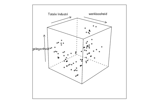
| Title produced by software | Trivariate Scatterplots | ||||||||||||||||||||
| Date of computation | Sun, 06 Jan 2008 12:39:26 -0700 | ||||||||||||||||||||
| Cite this page as follows | Statistical Computations at FreeStatistics.org, Office for Research Development and Education, URL https://freestatistics.org/blog/index.php?v=date/2008/Jan/06/t1199648377id7anr6d1y7s8zq.htm/, Retrieved Sat, 04 May 2024 22:39:39 +0000 | ||||||||||||||||||||
| Statistical Computations at FreeStatistics.org, Office for Research Development and Education, URL https://freestatistics.org/blog/index.php?pk=7866, Retrieved Sat, 04 May 2024 22:39:39 +0000 | |||||||||||||||||||||
| QR Codes: | |||||||||||||||||||||
|
| |||||||||||||||||||||
| Original text written by user: | |||||||||||||||||||||
| IsPrivate? | No (this computation is public) | ||||||||||||||||||||
| User-defined keywords | x totale industrie y werkgelegenheid z werkloosheid | ||||||||||||||||||||
| Estimated Impact | 149 | ||||||||||||||||||||
Tree of Dependent Computations | |||||||||||||||||||||
| Family? (F = Feedback message, R = changed R code, M = changed R Module, P = changed Parameters, D = changed Data) | |||||||||||||||||||||
| - [Central Tendency] [WS2 - Robustness ...] [2007-10-20 13:06:37] [5343e105a400b9e32bf6f011133bbaf4] - RM D [Trivariate Scatterplots] [CVWS5Q1C3] [2008-01-06 19:39:26] [b523c8d839cc24a05ea912c062a47207] [Current] | |||||||||||||||||||||
| Feedback Forum | |||||||||||||||||||||
Post a new message | |||||||||||||||||||||
Dataset | |||||||||||||||||||||
| Dataseries X: | |||||||||||||||||||||
-12.7 -2.4 7.1 -3.9 9.5 5 -16.1 -10.8 7 13.6 8.1 -8.1 4.9 -0.8 4.3 4 1.5 5.4 -11.3 -16.4 -2 8.9 -7.2 -18 1.3 6.3 -6 2.8 2 5.1 -7.6 -18.6 5.8 20.3 0.7 -11.2 -5.7 -0.1 3.4 3.3 -1.2 4.2 -8.8 -25.3 8.5 14.5 -3.1 -10.4 -2.9 0.3 22.6 15.4 9 29.1 2.8 -3.8 27.7 28.9 26.5 19.8 13.2 14.1 34.1 30 21.8 32.1 5.3 3 17.1 26.3 38.1 19.5 38 35.5 78.6 62.2 76.9 104.9 32.2 42.5 64.3 74.9 75.4 43 58.7 55.4 76.6 63.3 78.9 82.7 | |||||||||||||||||||||
| Dataseries Y: | |||||||||||||||||||||
59.9 59.9 59.9 60.9 60.9 60.9 61.1 61.1 61.1 60.2 60.2 60.2 60.1 60.1 60.1 59.7 59.7 59.7 60.5 60.5 60.5 59.5 59.5 59.5 59.5 59.5 59.5 59.7 59.7 59.7 60.4 60.4 60.4 60 60 60 59 59 59 59.3 59.3 59.3 59.7 59.7 59.7 60.4 60.4 60.4 59.9 59.9 59.9 60.5 60.5 60.5 60.4 60.4 60.4 60.6 60.6 60.6 60.9 60.9 60.9 61 61 61 61.2 61.2 61.2 61.2 61.2 61.2 60.3 60.3 60.3 60.4 60.4 60.4 61.2 61.2 61.2 62.1 62.1 62.1 61.7 61.7 61.7 61.6 61.6 61.6 | |||||||||||||||||||||
| Dataseries Z: | |||||||||||||||||||||
7,3 7,2 7,1 6,9 6,8 6,7 6,8 6,8 6,7 6,8 6,8 6,7 6,3 6,2 6,2 6,5 6,5 6,4 6,2 6,2 6,3 7,5 7,4 7,4 7,4 7,4 7,4 7,2 7,2 7,2 7,5 7,4 7,5 8,0 8,0 8,0 8,1 8,1 8,1 7,9 7,9 8,0 8,2 8,1 8,2 8,5 8,5 8,6 8,4 8,4 8,4 7,7 7,8 7,9 8,8 8,8 8,9 8,5 8,5 8,5 8,4 8,5 8,4 8,3 8,4 8,4 8,5 8,5 8,5 8,5 8,5 8,5 8,5 8,5 8,5 8,3 8,3 8,3 8,2 8,1 8,1 8,2 8,0 7,9 7,9 7,8 7,7 7,9 7,7 7,6 | |||||||||||||||||||||
Tables (Output of Computation) | |||||||||||||||||||||
| |||||||||||||||||||||
Figures (Output of Computation) | |||||||||||||||||||||
Input Parameters & R Code | |||||||||||||||||||||
| Parameters (Session): | |||||||||||||||||||||
| Parameters (R input): | |||||||||||||||||||||
| par1 = 50 ; par2 = 50 ; par3 = Y ; par4 = Y ; par5 = Totale Industri ; par6 = werkgelegenheid ; par7 = werkloosheid ; | |||||||||||||||||||||
| R code (references can be found in the software module): | |||||||||||||||||||||
x <- array(x,dim=c(length(x),1)) | |||||||||||||||||||||