Free Statistics
of Irreproducible Research!
Description of Statistical Computation | |||||||||||||||||||||
|---|---|---|---|---|---|---|---|---|---|---|---|---|---|---|---|---|---|---|---|---|---|
| Author's title | |||||||||||||||||||||
| Author | *Unverified author* | ||||||||||||||||||||
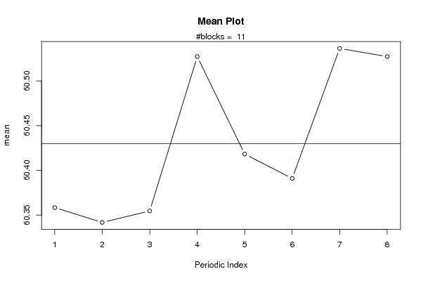
| R Software Module | rwasp_meanplot.wasp | ||||||||||||||||||||
| Title produced by software | Mean Plot | ||||||||||||||||||||
| Date of computation | Sun, 06 Jan 2008 10:13:00 -0700 | ||||||||||||||||||||
| Cite this page as follows | Statistical Computations at FreeStatistics.org, Office for Research Development and Education, URL https://freestatistics.org/blog/index.php?v=date/2008/Jan/06/t11996396522andcsc90npg4ud.htm/, Retrieved Sun, 05 May 2024 01:31:18 +0000 | ||||||||||||||||||||
| Statistical Computations at FreeStatistics.org, Office for Research Development and Education, URL https://freestatistics.org/blog/index.php?pk=7843, Retrieved Sun, 05 May 2024 01:31:18 +0000 | |||||||||||||||||||||
| QR Codes: | |||||||||||||||||||||
|
| |||||||||||||||||||||
| Original text written by user: | |||||||||||||||||||||
| IsPrivate? | No (this computation is public) | ||||||||||||||||||||
| User-defined keywords | Hypo testing with EDA Q2 Werkgelegenheid | ||||||||||||||||||||
| Estimated Impact | 186 | ||||||||||||||||||||
Tree of Dependent Computations | |||||||||||||||||||||
| Family? (F = Feedback message, R = changed R code, M = changed R Module, P = changed Parameters, D = changed Data) | |||||||||||||||||||||
| - [Central Tendency] [WS2 - Robustness ...] [2007-10-20 13:06:37] [5343e105a400b9e32bf6f011133bbaf4] - RM D [Mean Plot] [CVWS3WGQ2] [2008-01-06 17:13:00] [b523c8d839cc24a05ea912c062a47207] [Current] | |||||||||||||||||||||
| Feedback Forum | |||||||||||||||||||||
Post a new message | |||||||||||||||||||||
Dataset | |||||||||||||||||||||
| Dataseries X: | |||||||||||||||||||||
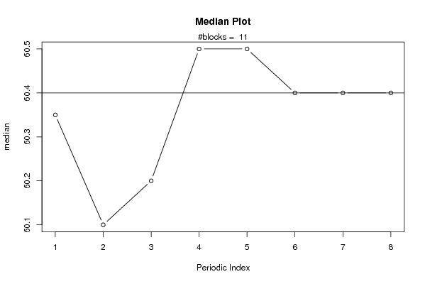
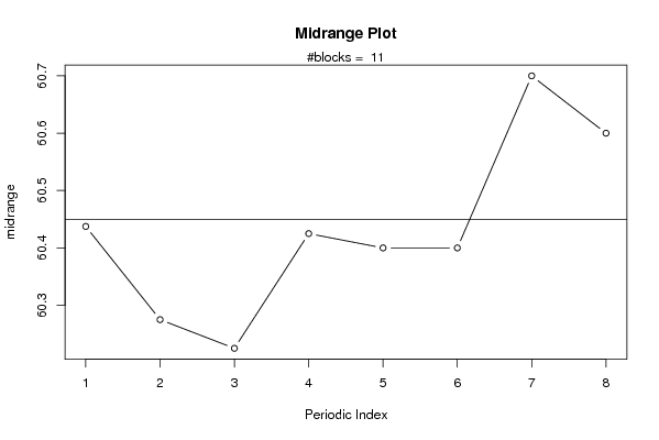
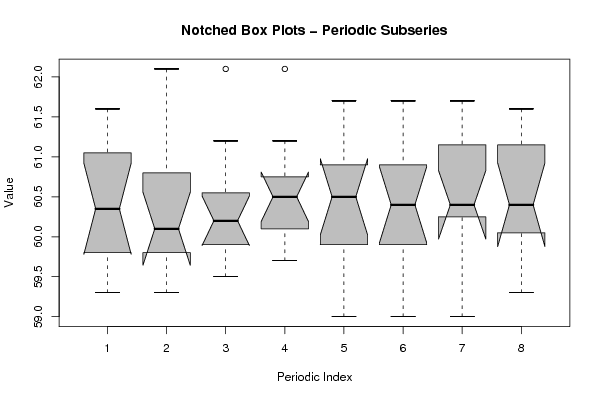
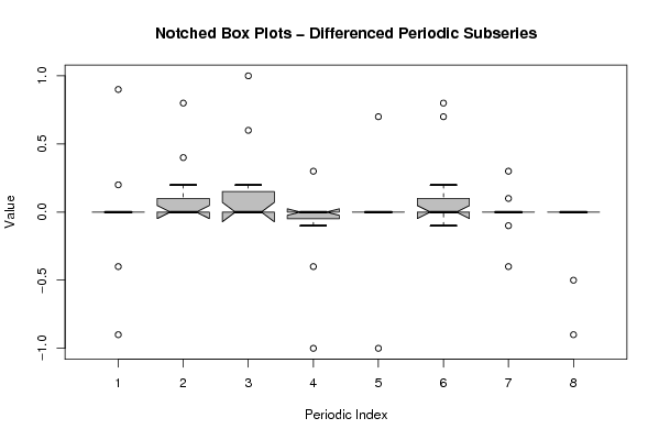
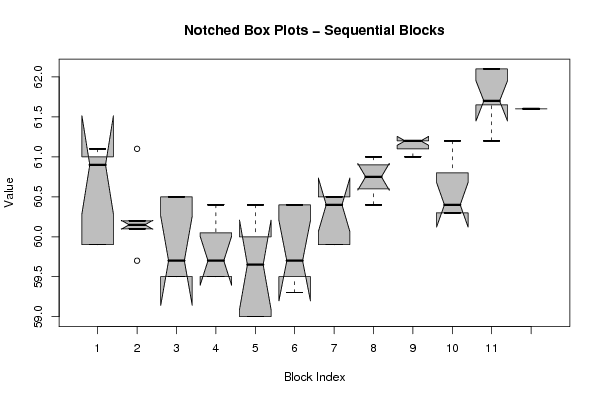
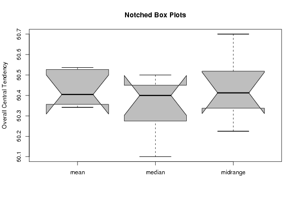
59.9 59.9 59.9 60.9 60.9 60.9 61.1 61.1 61.1 60.2 60.2 60.2 60.1 60.1 60.1 59.7 59.7 59.7 60.5 60.5 60.5 59.5 59.5 59.5 59.5 59.5 59.5 59.7 59.7 59.7 60.4 60.4 60.4 60 60 60 59 59 59 59.3 59.3 59.3 59.7 59.7 59.7 60.4 60.4 60.4 59.9 59.9 59.9 60.5 60.5 60.5 60.4 60.4 60.4 60.6 60.6 60.6 60.9 60.9 60.9 61 61 61 61.2 61.2 61.2 61.2 61.2 61.2 60.3 60.3 60.3 60.4 60.4 60.4 61.2 61.2 61.2 62.1 62.1 62.1 61.7 61.7 61.7 61.6 61.6 61.6 | |||||||||||||||||||||
Tables (Output of Computation) | |||||||||||||||||||||
| |||||||||||||||||||||
Figures (Output of Computation) | |||||||||||||||||||||
Input Parameters & R Code | |||||||||||||||||||||
| Parameters (Session): | |||||||||||||||||||||
| Parameters (R input): | |||||||||||||||||||||
| par1 = 8 ; | |||||||||||||||||||||
| R code (references can be found in the software module): | |||||||||||||||||||||
par1 <- as.numeric(par1) | |||||||||||||||||||||