Free Statistics
of Irreproducible Research!
Description of Statistical Computation | |||||||||||||||||||||||||||||||||||||||||||||||||||||
|---|---|---|---|---|---|---|---|---|---|---|---|---|---|---|---|---|---|---|---|---|---|---|---|---|---|---|---|---|---|---|---|---|---|---|---|---|---|---|---|---|---|---|---|---|---|---|---|---|---|---|---|---|---|
| Author's title | |||||||||||||||||||||||||||||||||||||||||||||||||||||
| Author | *Unverified author* | ||||||||||||||||||||||||||||||||||||||||||||||||||||
| R Software Module | rwasp_edauni.wasp | ||||||||||||||||||||||||||||||||||||||||||||||||||||
| Title produced by software | Univariate Explorative Data Analysis | ||||||||||||||||||||||||||||||||||||||||||||||||||||
| Date of computation | Sun, 06 Jan 2008 09:09:55 -0700 | ||||||||||||||||||||||||||||||||||||||||||||||||||||
| Cite this page as follows | Statistical Computations at FreeStatistics.org, Office for Research Development and Education, URL https://freestatistics.org/blog/index.php?v=date/2008/Jan/06/t1199635829z0fd34wel2k720k.htm/, Retrieved Sun, 05 May 2024 06:07:54 +0000 | ||||||||||||||||||||||||||||||||||||||||||||||||||||
| Statistical Computations at FreeStatistics.org, Office for Research Development and Education, URL https://freestatistics.org/blog/index.php?pk=7830, Retrieved Sun, 05 May 2024 06:07:54 +0000 | |||||||||||||||||||||||||||||||||||||||||||||||||||||
| QR Codes: | |||||||||||||||||||||||||||||||||||||||||||||||||||||
|
| |||||||||||||||||||||||||||||||||||||||||||||||||||||
| Original text written by user: | |||||||||||||||||||||||||||||||||||||||||||||||||||||
| IsPrivate? | No (this computation is public) | ||||||||||||||||||||||||||||||||||||||||||||||||||||
| User-defined keywords | Investigating distributions Werkgelegenheid Q2 | ||||||||||||||||||||||||||||||||||||||||||||||||||||
| Estimated Impact | 228 | ||||||||||||||||||||||||||||||||||||||||||||||||||||
Tree of Dependent Computations | |||||||||||||||||||||||||||||||||||||||||||||||||||||
| Family? (F = Feedback message, R = changed R code, M = changed R Module, P = changed Parameters, D = changed Data) | |||||||||||||||||||||||||||||||||||||||||||||||||||||
| - [Central Tendency] [WS2 - Robustness ...] [2007-10-20 13:06:37] [5343e105a400b9e32bf6f011133bbaf4] - RM D [Univariate Explorative Data Analysis] [CVWS2WGQ2] [2008-01-06 16:09:55] [d41d8cd98f00b204e9800998ecf8427e] [Current] - PD [Univariate Explorative Data Analysis] [CVWS2Q21] [2008-01-16 22:20:11] [74be16979710d4c4e7c6647856088456] - PD [Univariate Explorative Data Analysis] [cvws2q22] [2008-01-16 22:41:38] [74be16979710d4c4e7c6647856088456] - RMPD [Cronbach Alpha] [Question 2 - Extr...] [2010-10-19 22:07:18] [b9f5bf8f9089a40337275cf2fd2f13a1] - D [Cronbach Alpha] [Question 2 - Extr...] [2010-10-19 22:12:56] [b9f5bf8f9089a40337275cf2fd2f13a1] - D [Cronbach Alpha] [Question 2 - Extr...] [2010-10-19 22:35:49] [b9f5bf8f9089a40337275cf2fd2f13a1] - D [Cronbach Alpha] [Question 2 - Extr...] [2010-10-19 22:43:00] [b9f5bf8f9089a40337275cf2fd2f13a1] - PD [Univariate Explorative Data Analysis] [cvws2q23] [2008-01-16 22:46:36] [74be16979710d4c4e7c6647856088456] - PD [Univariate Explorative Data Analysis] [cvws2q24] [2008-01-16 22:51:16] [74be16979710d4c4e7c6647856088456] | |||||||||||||||||||||||||||||||||||||||||||||||||||||
| Feedback Forum | |||||||||||||||||||||||||||||||||||||||||||||||||||||
Post a new message | |||||||||||||||||||||||||||||||||||||||||||||||||||||
Dataset | |||||||||||||||||||||||||||||||||||||||||||||||||||||
| Dataseries X: | |||||||||||||||||||||||||||||||||||||||||||||||||||||
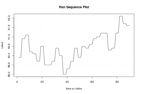
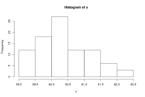
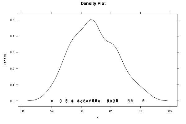
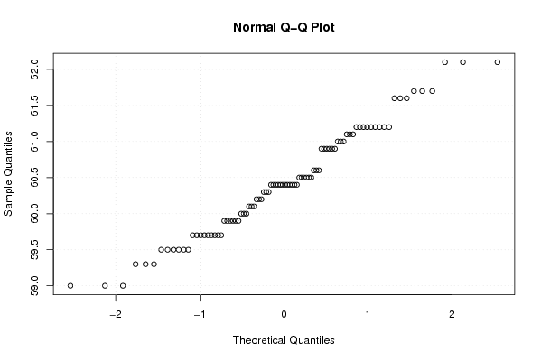
59.9 59.9 59.9 60.9 60.9 60.9 61.1 61.1 61.1 60.2 60.2 60.2 60.1 60.1 60.1 59.7 59.7 59.7 60.5 60.5 60.5 59.5 59.5 59.5 59.5 59.5 59.5 59.7 59.7 59.7 60.4 60.4 60.4 60 60 60 59 59 59 59.3 59.3 59.3 59.7 59.7 59.7 60.4 60.4 60.4 59.9 59.9 59.9 60.5 60.5 60.5 60.4 60.4 60.4 60.6 60.6 60.6 60.9 60.9 60.9 61 61 61 61.2 61.2 61.2 61.2 61.2 61.2 60.3 60.3 60.3 60.4 60.4 60.4 61.2 61.2 61.2 62.1 62.1 62.1 61.7 61.7 61.7 61.6 61.6 61.6 | |||||||||||||||||||||||||||||||||||||||||||||||||||||
Tables (Output of Computation) | |||||||||||||||||||||||||||||||||||||||||||||||||||||
| |||||||||||||||||||||||||||||||||||||||||||||||||||||
Figures (Output of Computation) | |||||||||||||||||||||||||||||||||||||||||||||||||||||
Input Parameters & R Code | |||||||||||||||||||||||||||||||||||||||||||||||||||||
| Parameters (Session): | |||||||||||||||||||||||||||||||||||||||||||||||||||||
| Parameters (R input): | |||||||||||||||||||||||||||||||||||||||||||||||||||||
| par1 = 0 ; par2 = 0 ; | |||||||||||||||||||||||||||||||||||||||||||||||||||||
| R code (references can be found in the software module): | |||||||||||||||||||||||||||||||||||||||||||||||||||||
par1 <- as.numeric(par1) | |||||||||||||||||||||||||||||||||||||||||||||||||||||