Free Statistics
of Irreproducible Research!
Description of Statistical Computation | |||||||||||||||||||||
|---|---|---|---|---|---|---|---|---|---|---|---|---|---|---|---|---|---|---|---|---|---|
| Author's title | |||||||||||||||||||||
| Author | *The author of this computation has been verified* | ||||||||||||||||||||
| R Software Module | rwasp_meanplot.wasp | ||||||||||||||||||||
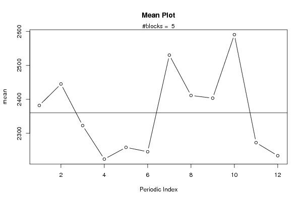
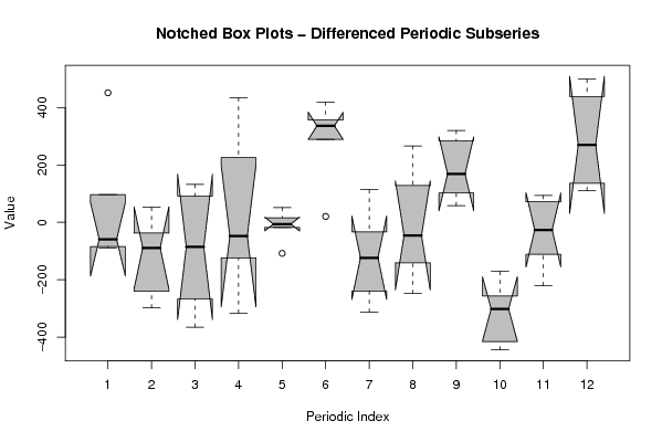
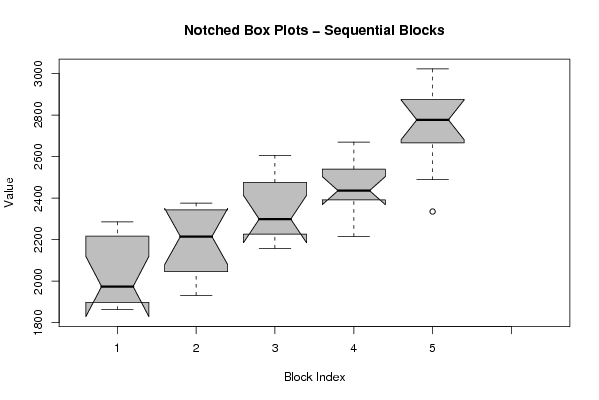
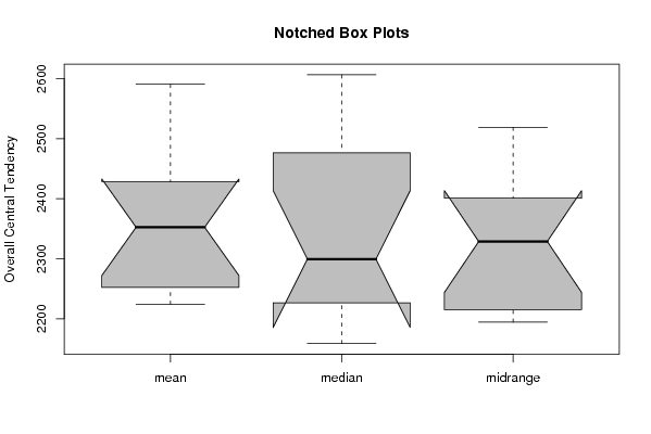
| Title produced by software | Mean Plot | ||||||||||||||||||||
| Date of computation | Mon, 22 Dec 2008 06:33:34 -0700 | ||||||||||||||||||||
| Cite this page as follows | Statistical Computations at FreeStatistics.org, Office for Research Development and Education, URL https://freestatistics.org/blog/index.php?v=date/2008/Dec/22/t12299528816snsvn3ehicfi1r.htm/, Retrieved Sun, 12 May 2024 12:38:54 +0000 | ||||||||||||||||||||
| Statistical Computations at FreeStatistics.org, Office for Research Development and Education, URL https://freestatistics.org/blog/index.php?pk=36056, Retrieved Sun, 12 May 2024 12:38:54 +0000 | |||||||||||||||||||||
| QR Codes: | |||||||||||||||||||||
|
| |||||||||||||||||||||
| Original text written by user: | |||||||||||||||||||||
| IsPrivate? | No (this computation is public) | ||||||||||||||||||||
| User-defined keywords | |||||||||||||||||||||
| Estimated Impact | 186 | ||||||||||||||||||||
Tree of Dependent Computations | |||||||||||||||||||||
| Family? (F = Feedback message, R = changed R code, M = changed R Module, P = changed Parameters, D = changed Data) | |||||||||||||||||||||
| F [Univariate Data Series] [Airline data] [2007-10-18 09:58:47] [42daae401fd3def69a25014f2252b4c2] - R PD [Univariate Data Series] [Tijdreeks 2 Buite...] [2008-12-11 16:25:30] [2d4aec5ed1856c4828162be37be304d9] - RMP [Central Tendency] [Central tendency ...] [2008-12-11 17:41:16] [2d4aec5ed1856c4828162be37be304d9] - RMP [Blocked Bootstrap Plot - Central Tendency] [Blocked Bootstrap...] [2008-12-12 08:14:08] [2d4aec5ed1856c4828162be37be304d9] - RMP [Tukey lambda PPCC Plot] [Tukey Lambda PPCC...] [2008-12-12 08:45:26] [2d4aec5ed1856c4828162be37be304d9] - RMP [Standard Deviation-Mean Plot] [SD Mean Plot Tijd...] [2008-12-12 09:35:09] [2d4aec5ed1856c4828162be37be304d9] - RMP [Box-Cox Normality Plot] [Box-Cox Normality...] [2008-12-12 09:46:16] [2d4aec5ed1856c4828162be37be304d9] - RMP [Mean Plot] [Mean plot Yt] [2008-12-22 13:33:34] [d7f41258beeebb8716e3f5d39f3cdc01] [Current] | |||||||||||||||||||||
| Feedback Forum | |||||||||||||||||||||
Post a new message | |||||||||||||||||||||
Dataset | |||||||||||||||||||||
| Dataseries X: | |||||||||||||||||||||
2220.6 2161.5 1863.6 1955.1 1907.4 1889.4 2246.3 2213 1965 2285.6 1983.8 1872.4 2371.4 2287 2198.2 2330.4 2014.4 2066.1 2355.8 2232.5 2091.7 2376.5 1931.9 2025.7 2404.9 2316.1 2368.1 2282.5 2158.6 2174.8 2594.1 2281.4 2547.9 2606.3 2190.8 2262.3 2423.8 2520.4 2482.9 2215.9 2441.9 2333.8 2670.2 2431 2559.3 2661.4 2404.6 2378.3 2489.2 2941 2700.9 2335.6 2770 2764.2 2784.9 2898.8 2853.4 3022.6 2851.4 2630.8 | |||||||||||||||||||||
Tables (Output of Computation) | |||||||||||||||||||||
| |||||||||||||||||||||
Figures (Output of Computation) | |||||||||||||||||||||
Input Parameters & R Code | |||||||||||||||||||||
| Parameters (Session): | |||||||||||||||||||||
| par1 = 12 ; | |||||||||||||||||||||
| Parameters (R input): | |||||||||||||||||||||
| par1 = 12 ; | |||||||||||||||||||||
| R code (references can be found in the software module): | |||||||||||||||||||||
par1 <- as.numeric(par1) | |||||||||||||||||||||