Repository of Reproducible Computations

Free Statistics

of Irreproducible Research!

Author's title

Author

*The author of this computation has been verified*

R Software Module

rwasp_arimaforecasting.wasp

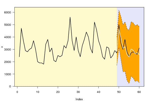
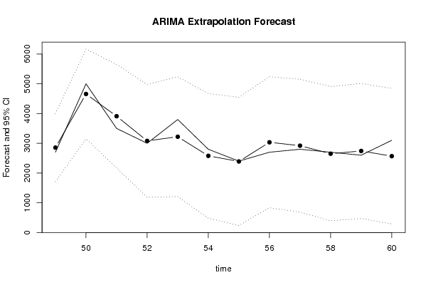
Title produced by software

ARIMA Forecasting

Date of computation

Mon, 22 Dec 2008 06:06:40 -0700

Cite this page as follows

Statistical Computations at FreeStatistics.org, Office for Research Development and Education, URL https://freestatistics.org/blog/index.php?v=date/2008/Dec/22/t1229951621s8fxfzf8lh72clv.htm/, Retrieved Sun, 12 May 2024 21:45:46 +0000

Statistical Computations at FreeStatistics.org, Office for Research Development and Education, URL https://freestatistics.org/blog/index.php?pk=36043, Retrieved Sun, 12 May 2024 21:45:46 +0000

QR Codes:

Paste this QR Code to cite your computation.

Original text written by user:

In samenwerking met Katrien Bourdiaudhy, St�phanie Claes en Kevin Engels

IsPrivate?

No (this computation is public)

User-defined keywords

Estimated Impact

192

Family? (F = Feedback message, R = changed R code, M = changed R Module, P = changed Parameters, D = changed Data)

F     [Univariate Data Series] [blog 1e tijdreeks...] [2008-10-13 19:23:31] [7173087adebe3e3a714c80ea2417b3eb]
-   PD  [Univariate Data Series] [tijdreeksen opnie...] [2008-10-19 17:18:46] [7173087adebe3e3a714c80ea2417b3eb]
- RMP     [Central Tendency] [tijdreeks 2 centr...] [2008-10-19 17:39:42] [7173087adebe3e3a714c80ea2417b3eb]
- RMP       [(Partial) Autocorrelation Function] [ACF aanvragen hyp...] [2008-12-16 14:51:47] [7d3039e6253bb5fb3b26df1537d500b4]
- RMP         [ARIMA Backward Selection] [Arima backward aa...] [2008-12-16 15:38:56] [7d3039e6253bb5fb3b26df1537d500b4]
- RMP           [(Partial) Autocorrelation Function] [acf hypothecair k...] [2008-12-17 15:13:05] [7173087adebe3e3a714c80ea2417b3eb]
- RMP             [ARIMA Backward Selection] [Arima backward se...] [2008-12-17 19:36:16] [7d3039e6253bb5fb3b26df1537d500b4]
-   P               [ARIMA Backward Selection] [Arima aanvragen h...] [2008-12-18 11:08:22] [7d3039e6253bb5fb3b26df1537d500b4]
- RMP                   [ARIMA Forecasting] [forecast aantal a...] [2008-12-22 13:06:40] [95d95b0e883740fcbc85e18ec42dcafb] [Current]

Feedback Forum

Post a new message

Dataseries X:

Download CSV

Histogram

Boxplots

Summary of computational transaction
Raw Input	view raw input (R code)
Raw Output	view raw output of R engine
Computing time	1 seconds
R Server	'Gwilym Jenkins' @ 72.249.127.135

\begin{tabular}{lllllllll}
\hline
Summary of computational transaction \tabularnewline
Raw Input & view raw input (R code)  \tabularnewline
Raw Output & view raw output of R engine  \tabularnewline
Computing time & 1 seconds \tabularnewline
R Server & 'Gwilym Jenkins' @ 72.249.127.135 \tabularnewline
\hline
\end{tabular}
%Source: https://freestatistics.org/blog/index.php?pk=36043&T=0

[TABLE]
[ROW][C]Summary of computational transaction[/C][/ROW]
[ROW][C]Raw Input[/C][C]view raw input (R code) [/C][/ROW]
[ROW][C]Raw Output[/C][C]view raw output of R engine [/C][/ROW]
[ROW][C]Computing time[/C][C]1 seconds[/C][/ROW]
[ROW][C]R Server[/C][C]'Gwilym Jenkins' @ 72.249.127.135[/C][/ROW]
[/TABLE]
Source: https://freestatistics.org/blog/index.php?pk=36043&T=0

Globally Unique Identifier (entire table): ba.freestatistics.org/blog/index.php?pk=36043&T=0

As an alternative you can also use a QR Code:

The GUIDs for individual cells are displayed in the table below:

Summary of computational transaction
Raw Input	view raw input (R code)
Raw Output	view raw output of R engine
Computing time	1 seconds
R Server	'Gwilym Jenkins' @ 72.249.127.135

Univariate ARIMA Extrapolation Forecast
time	Y[t]	F[t]	95% LB	95% UB	p-value(H0: Y[t] = F[t])	P(F[t]>Y[t-1])	P(F[t]>Y[t-s])	P(F[t]>Y[48])
36	3100	-	-	-	-	-	-	-
37	2700	-	-	-	-	-	-	-
38	5200	-	-	-	-	-	-	-
39	4600	-	-	-	-	-	-	-
40	3700	-	-	-	-	-	-	-
41	3200	-	-	-	-	-	-	-
42	2400	-	-	-	-	-	-	-
43	2200	-	-	-	-	-	-	-
44	3200	-	-	-	-	-	-	-
45	3100	-	-	-	-	-	-	-
46	2300	-	-	-	-	-	-	-
47	2500	-	-	-	-	-	-	-
48	2900	-	-	-	-	-	-	-
49	2700	2855.881	1711.4942	4000.2679	0.3947	0.4699	0.6053	0.4699
50	5000	4658.5269	3150.1212	6166.9327	0.3286	0.9945	0.2408	0.9888
51	3500	3912.0172	2173.1109	5650.9234	0.3212	0.11	0.219	0.873
52	3000	3082.2635	1184.1109	4980.4161	0.4662	0.3331	0.2618	0.5746
53	3800	3220.6933	1208.2639	5233.1227	0.2863	0.5851	0.508	0.6226
54	2800	2578.8069	482.8526	4674.7613	0.4181	0.1267	0.5664	0.382
55	2400	2389.6862	232.2866	4547.0859	0.4963	0.3547	0.5684	0.3215
56	2700	3034.4363	832.0234	5236.8491	0.383	0.7138	0.4414	0.5476
57	2800	2920.355	685.5585	5155.1515	0.458	0.5766	0.4374	0.5071
58	2700	2651.1354	394.0053	4908.2655	0.4831	0.4486	0.6198	0.4145
59	2600	2742.5096	471.3871	5013.632	0.4511	0.5146	0.5829	0.4459
60	3100	2567.6302	289.8137	4845.4467	0.3234	0.4889	0.3874	0.3874

\begin{tabular}{lllllllll}
\hline
Univariate ARIMA Extrapolation Forecast \tabularnewline
time & Y[t] & F[t] & 95% LB & 95% UB & p-value(H0: Y[t] = F[t]) & P(F[t]>Y[t-1]) & P(F[t]>Y[t-s]) & P(F[t]>Y[48]) \tabularnewline
36 & 3100 & - & - & - & - & - & - & - \tabularnewline
37 & 2700 & - & - & - & - & - & - & - \tabularnewline
38 & 5200 & - & - & - & - & - & - & - \tabularnewline
39 & 4600 & - & - & - & - & - & - & - \tabularnewline
40 & 3700 & - & - & - & - & - & - & - \tabularnewline
41 & 3200 & - & - & - & - & - & - & - \tabularnewline
42 & 2400 & - & - & - & - & - & - & - \tabularnewline
43 & 2200 & - & - & - & - & - & - & - \tabularnewline
44 & 3200 & - & - & - & - & - & - & - \tabularnewline
45 & 3100 & - & - & - & - & - & - & - \tabularnewline
46 & 2300 & - & - & - & - & - & - & - \tabularnewline
47 & 2500 & - & - & - & - & - & - & - \tabularnewline
48 & 2900 & - & - & - & - & - & - & - \tabularnewline
49 & 2700 & 2855.881 & 1711.4942 & 4000.2679 & 0.3947 & 0.4699 & 0.6053 & 0.4699 \tabularnewline
50 & 5000 & 4658.5269 & 3150.1212 & 6166.9327 & 0.3286 & 0.9945 & 0.2408 & 0.9888 \tabularnewline
51 & 3500 & 3912.0172 & 2173.1109 & 5650.9234 & 0.3212 & 0.11 & 0.219 & 0.873 \tabularnewline
52 & 3000 & 3082.2635 & 1184.1109 & 4980.4161 & 0.4662 & 0.3331 & 0.2618 & 0.5746 \tabularnewline
53 & 3800 & 3220.6933 & 1208.2639 & 5233.1227 & 0.2863 & 0.5851 & 0.508 & 0.6226 \tabularnewline
54 & 2800 & 2578.8069 & 482.8526 & 4674.7613 & 0.4181 & 0.1267 & 0.5664 & 0.382 \tabularnewline
55 & 2400 & 2389.6862 & 232.2866 & 4547.0859 & 0.4963 & 0.3547 & 0.5684 & 0.3215 \tabularnewline
56 & 2700 & 3034.4363 & 832.0234 & 5236.8491 & 0.383 & 0.7138 & 0.4414 & 0.5476 \tabularnewline
57 & 2800 & 2920.355 & 685.5585 & 5155.1515 & 0.458 & 0.5766 & 0.4374 & 0.5071 \tabularnewline
58 & 2700 & 2651.1354 & 394.0053 & 4908.2655 & 0.4831 & 0.4486 & 0.6198 & 0.4145 \tabularnewline
59 & 2600 & 2742.5096 & 471.3871 & 5013.632 & 0.4511 & 0.5146 & 0.5829 & 0.4459 \tabularnewline
60 & 3100 & 2567.6302 & 289.8137 & 4845.4467 & 0.3234 & 0.4889 & 0.3874 & 0.3874 \tabularnewline
\hline
\end{tabular}
%Source: https://freestatistics.org/blog/index.php?pk=36043&T=1

[TABLE]
[ROW][C]Univariate ARIMA Extrapolation Forecast[/C][/ROW]
[ROW][C]time[/C][C]Y[t][/C][C]F[t][/C][C]95% LB[/C][C]95% UB[/C][C]p-value(H0: Y[t] = F[t])[/C][C]P(F[t]>Y[t-1])[/C][C]P(F[t]>Y[t-s])[/C][C]P(F[t]>Y[48])[/C][/ROW]
[ROW][C]36[/C][C]3100[/C][C]-[/C][C]-[/C][C]-[/C][C]-[/C][C]-[/C][C]-[/C][C]-[/C][/ROW]
[ROW][C]37[/C][C]2700[/C][C]-[/C][C]-[/C][C]-[/C][C]-[/C][C]-[/C][C]-[/C][C]-[/C][/ROW]
[ROW][C]38[/C][C]5200[/C][C]-[/C][C]-[/C][C]-[/C][C]-[/C][C]-[/C][C]-[/C][C]-[/C][/ROW]
[ROW][C]39[/C][C]4600[/C][C]-[/C][C]-[/C][C]-[/C][C]-[/C][C]-[/C][C]-[/C][C]-[/C][/ROW]
[ROW][C]40[/C][C]3700[/C][C]-[/C][C]-[/C][C]-[/C][C]-[/C][C]-[/C][C]-[/C][C]-[/C][/ROW]
[ROW][C]41[/C][C]3200[/C][C]-[/C][C]-[/C][C]-[/C][C]-[/C][C]-[/C][C]-[/C][C]-[/C][/ROW]
[ROW][C]42[/C][C]2400[/C][C]-[/C][C]-[/C][C]-[/C][C]-[/C][C]-[/C][C]-[/C][C]-[/C][/ROW]
[ROW][C]43[/C][C]2200[/C][C]-[/C][C]-[/C][C]-[/C][C]-[/C][C]-[/C][C]-[/C][C]-[/C][/ROW]
[ROW][C]44[/C][C]3200[/C][C]-[/C][C]-[/C][C]-[/C][C]-[/C][C]-[/C][C]-[/C][C]-[/C][/ROW]
[ROW][C]45[/C][C]3100[/C][C]-[/C][C]-[/C][C]-[/C][C]-[/C][C]-[/C][C]-[/C][C]-[/C][/ROW]
[ROW][C]46[/C][C]2300[/C][C]-[/C][C]-[/C][C]-[/C][C]-[/C][C]-[/C][C]-[/C][C]-[/C][/ROW]
[ROW][C]47[/C][C]2500[/C][C]-[/C][C]-[/C][C]-[/C][C]-[/C][C]-[/C][C]-[/C][C]-[/C][/ROW]
[ROW][C]48[/C][C]2900[/C][C]-[/C][C]-[/C][C]-[/C][C]-[/C][C]-[/C][C]-[/C][C]-[/C][/ROW]
[ROW][C]49[/C][C]2700[/C][C]2855.881[/C][C]1711.4942[/C][C]4000.2679[/C][C]0.3947[/C][C]0.4699[/C][C]0.6053[/C][C]0.4699[/C][/ROW]
[ROW][C]50[/C][C]5000[/C][C]4658.5269[/C][C]3150.1212[/C][C]6166.9327[/C][C]0.3286[/C][C]0.9945[/C][C]0.2408[/C][C]0.9888[/C][/ROW]
[ROW][C]51[/C][C]3500[/C][C]3912.0172[/C][C]2173.1109[/C][C]5650.9234[/C][C]0.3212[/C][C]0.11[/C][C]0.219[/C][C]0.873[/C][/ROW]
[ROW][C]52[/C][C]3000[/C][C]3082.2635[/C][C]1184.1109[/C][C]4980.4161[/C][C]0.4662[/C][C]0.3331[/C][C]0.2618[/C][C]0.5746[/C][/ROW]
[ROW][C]53[/C][C]3800[/C][C]3220.6933[/C][C]1208.2639[/C][C]5233.1227[/C][C]0.2863[/C][C]0.5851[/C][C]0.508[/C][C]0.6226[/C][/ROW]
[ROW][C]54[/C][C]2800[/C][C]2578.8069[/C][C]482.8526[/C][C]4674.7613[/C][C]0.4181[/C][C]0.1267[/C][C]0.5664[/C][C]0.382[/C][/ROW]
[ROW][C]55[/C][C]2400[/C][C]2389.6862[/C][C]232.2866[/C][C]4547.0859[/C][C]0.4963[/C][C]0.3547[/C][C]0.5684[/C][C]0.3215[/C][/ROW]
[ROW][C]56[/C][C]2700[/C][C]3034.4363[/C][C]832.0234[/C][C]5236.8491[/C][C]0.383[/C][C]0.7138[/C][C]0.4414[/C][C]0.5476[/C][/ROW]
[ROW][C]57[/C][C]2800[/C][C]2920.355[/C][C]685.5585[/C][C]5155.1515[/C][C]0.458[/C][C]0.5766[/C][C]0.4374[/C][C]0.5071[/C][/ROW]
[ROW][C]58[/C][C]2700[/C][C]2651.1354[/C][C]394.0053[/C][C]4908.2655[/C][C]0.4831[/C][C]0.4486[/C][C]0.6198[/C][C]0.4145[/C][/ROW]
[ROW][C]59[/C][C]2600[/C][C]2742.5096[/C][C]471.3871[/C][C]5013.632[/C][C]0.4511[/C][C]0.5146[/C][C]0.5829[/C][C]0.4459[/C][/ROW]
[ROW][C]60[/C][C]3100[/C][C]2567.6302[/C][C]289.8137[/C][C]4845.4467[/C][C]0.3234[/C][C]0.4889[/C][C]0.3874[/C][C]0.3874[/C][/ROW]
[/TABLE]
Source: https://freestatistics.org/blog/index.php?pk=36043&T=1

Globally Unique Identifier (entire table): ba.freestatistics.org/blog/index.php?pk=36043&T=1

As an alternative you can also use a QR Code:

The GUIDs for individual cells are displayed in the table below:

Univariate ARIMA Extrapolation Forecast
time	Y[t]	F[t]	95% LB	95% UB	p-value(H0: Y[t] = F[t])	P(F[t]>Y[t-1])	P(F[t]>Y[t-s])	P(F[t]>Y[48])
36	3100	-	-	-	-	-	-	-
37	2700	-	-	-	-	-	-	-
38	5200	-	-	-	-	-	-	-
39	4600	-	-	-	-	-	-	-
40	3700	-	-	-	-	-	-	-
41	3200	-	-	-	-	-	-	-
42	2400	-	-	-	-	-	-	-
43	2200	-	-	-	-	-	-	-
44	3200	-	-	-	-	-	-	-
45	3100	-	-	-	-	-	-	-
46	2300	-	-	-	-	-	-	-
47	2500	-	-	-	-	-	-	-
48	2900	-	-	-	-	-	-	-
49	2700	2855.881	1711.4942	4000.2679	0.3947	0.4699	0.6053	0.4699
50	5000	4658.5269	3150.1212	6166.9327	0.3286	0.9945	0.2408	0.9888
51	3500	3912.0172	2173.1109	5650.9234	0.3212	0.11	0.219	0.873
52	3000	3082.2635	1184.1109	4980.4161	0.4662	0.3331	0.2618	0.5746
53	3800	3220.6933	1208.2639	5233.1227	0.2863	0.5851	0.508	0.6226
54	2800	2578.8069	482.8526	4674.7613	0.4181	0.1267	0.5664	0.382
55	2400	2389.6862	232.2866	4547.0859	0.4963	0.3547	0.5684	0.3215
56	2700	3034.4363	832.0234	5236.8491	0.383	0.7138	0.4414	0.5476
57	2800	2920.355	685.5585	5155.1515	0.458	0.5766	0.4374	0.5071
58	2700	2651.1354	394.0053	4908.2655	0.4831	0.4486	0.6198	0.4145
59	2600	2742.5096	471.3871	5013.632	0.4511	0.5146	0.5829	0.4459
60	3100	2567.6302	289.8137	4845.4467	0.3234	0.4889	0.3874	0.3874

Univariate ARIMA Extrapolation Forecast Performance
time	% S.E.	PE	MAPE	Sq.E	MSE	RMSE
49	0.2044	-0.0546	0.0045	24298.9008	2024.9084	44.999
50	0.1652	0.0733	0.0061	116603.8472	9716.9873	98.5748
51	0.2268	-0.1053	0.0088	169758.1579	14146.5132	118.9391
52	0.3142	-0.0267	0.0022	6767.2896	563.9408	23.7474
53	0.3188	0.1799	0.015	335596.2588	27966.3549	167.2314
54	0.4147	0.0858	0.0071	48926.375	4077.1979	63.8529
55	0.4606	0.0043	4e-04	106.3737	8.8645	2.9773
56	0.3703	-0.1102	0.0092	111847.6119	9320.6343	96.5434
57	0.3904	-0.0412	0.0034	14485.3253	1207.1104	34.7435
58	0.4344	0.0184	0.0015	2387.7522	198.9794	14.106
59	0.4225	-0.052	0.0043	20308.9731	1692.4144	41.139
60	0.4526	0.2073	0.0173	283417.5913	23618.1326	153.6819

\begin{tabular}{lllllllll}
\hline
Univariate ARIMA Extrapolation Forecast Performance \tabularnewline
time & % S.E. & PE & MAPE & Sq.E & MSE & RMSE \tabularnewline
49 & 0.2044 & -0.0546 & 0.0045 & 24298.9008 & 2024.9084 & 44.999 \tabularnewline
50 & 0.1652 & 0.0733 & 0.0061 & 116603.8472 & 9716.9873 & 98.5748 \tabularnewline
51 & 0.2268 & -0.1053 & 0.0088 & 169758.1579 & 14146.5132 & 118.9391 \tabularnewline
52 & 0.3142 & -0.0267 & 0.0022 & 6767.2896 & 563.9408 & 23.7474 \tabularnewline
53 & 0.3188 & 0.1799 & 0.015 & 335596.2588 & 27966.3549 & 167.2314 \tabularnewline
54 & 0.4147 & 0.0858 & 0.0071 & 48926.375 & 4077.1979 & 63.8529 \tabularnewline
55 & 0.4606 & 0.0043 & 4e-04 & 106.3737 & 8.8645 & 2.9773 \tabularnewline
56 & 0.3703 & -0.1102 & 0.0092 & 111847.6119 & 9320.6343 & 96.5434 \tabularnewline
57 & 0.3904 & -0.0412 & 0.0034 & 14485.3253 & 1207.1104 & 34.7435 \tabularnewline
58 & 0.4344 & 0.0184 & 0.0015 & 2387.7522 & 198.9794 & 14.106 \tabularnewline
59 & 0.4225 & -0.052 & 0.0043 & 20308.9731 & 1692.4144 & 41.139 \tabularnewline
60 & 0.4526 & 0.2073 & 0.0173 & 283417.5913 & 23618.1326 & 153.6819 \tabularnewline
\hline
\end{tabular}
%Source: https://freestatistics.org/blog/index.php?pk=36043&T=2

[TABLE]
[ROW][C]Univariate ARIMA Extrapolation Forecast Performance[/C][/ROW]
[ROW][C]time[/C][C]% S.E.[/C][C]PE[/C][C]MAPE[/C][C]Sq.E[/C][C]MSE[/C][C]RMSE[/C][/ROW]
[ROW][C]49[/C][C]0.2044[/C][C]-0.0546[/C][C]0.0045[/C][C]24298.9008[/C][C]2024.9084[/C][C]44.999[/C][/ROW]
[ROW][C]50[/C][C]0.1652[/C][C]0.0733[/C][C]0.0061[/C][C]116603.8472[/C][C]9716.9873[/C][C]98.5748[/C][/ROW]
[ROW][C]51[/C][C]0.2268[/C][C]-0.1053[/C][C]0.0088[/C][C]169758.1579[/C][C]14146.5132[/C][C]118.9391[/C][/ROW]
[ROW][C]52[/C][C]0.3142[/C][C]-0.0267[/C][C]0.0022[/C][C]6767.2896[/C][C]563.9408[/C][C]23.7474[/C][/ROW]
[ROW][C]53[/C][C]0.3188[/C][C]0.1799[/C][C]0.015[/C][C]335596.2588[/C][C]27966.3549[/C][C]167.2314[/C][/ROW]
[ROW][C]54[/C][C]0.4147[/C][C]0.0858[/C][C]0.0071[/C][C]48926.375[/C][C]4077.1979[/C][C]63.8529[/C][/ROW]
[ROW][C]55[/C][C]0.4606[/C][C]0.0043[/C][C]4e-04[/C][C]106.3737[/C][C]8.8645[/C][C]2.9773[/C][/ROW]
[ROW][C]56[/C][C]0.3703[/C][C]-0.1102[/C][C]0.0092[/C][C]111847.6119[/C][C]9320.6343[/C][C]96.5434[/C][/ROW]
[ROW][C]57[/C][C]0.3904[/C][C]-0.0412[/C][C]0.0034[/C][C]14485.3253[/C][C]1207.1104[/C][C]34.7435[/C][/ROW]
[ROW][C]58[/C][C]0.4344[/C][C]0.0184[/C][C]0.0015[/C][C]2387.7522[/C][C]198.9794[/C][C]14.106[/C][/ROW]
[ROW][C]59[/C][C]0.4225[/C][C]-0.052[/C][C]0.0043[/C][C]20308.9731[/C][C]1692.4144[/C][C]41.139[/C][/ROW]
[ROW][C]60[/C][C]0.4526[/C][C]0.2073[/C][C]0.0173[/C][C]283417.5913[/C][C]23618.1326[/C][C]153.6819[/C][/ROW]
[/TABLE]
Source: https://freestatistics.org/blog/index.php?pk=36043&T=2

Globally Unique Identifier (entire table): ba.freestatistics.org/blog/index.php?pk=36043&T=2

As an alternative you can also use a QR Code:

The GUIDs for individual cells are displayed in the table below:

Univariate ARIMA Extrapolation Forecast Performance
time	% S.E.	PE	MAPE	Sq.E	MSE	RMSE
49	0.2044	-0.0546	0.0045	24298.9008	2024.9084	44.999
50	0.1652	0.0733	0.0061	116603.8472	9716.9873	98.5748
51	0.2268	-0.1053	0.0088	169758.1579	14146.5132	118.9391
52	0.3142	-0.0267	0.0022	6767.2896	563.9408	23.7474
53	0.3188	0.1799	0.015	335596.2588	27966.3549	167.2314
54	0.4147	0.0858	0.0071	48926.375	4077.1979	63.8529
55	0.4606	0.0043	4e-04	106.3737	8.8645	2.9773
56	0.3703	-0.1102	0.0092	111847.6119	9320.6343	96.5434
57	0.3904	-0.0412	0.0034	14485.3253	1207.1104	34.7435
58	0.4344	0.0184	0.0015	2387.7522	198.9794	14.106
59	0.4225	-0.052	0.0043	20308.9731	1692.4144	41.139
60	0.4526	0.2073	0.0173	283417.5913	23618.1326	153.6819

Figure 1

PNG link

Postscript link

PDF link

Figure 2

PNG link

Postscript link

PDF link

Parameters (Session):

par1 = 12 ; par2 = 1 ; par3 = 0 ; par4 = 0 ; par5 = 12 ; par6 = 1 ; par7 = 0 ; par8 = 1 ; par9 = 1 ; par10 = FALSE ;

Parameters (R input):

par1 = 12 ; par2 = 1 ; par3 = 0 ; par4 = 0 ; par5 = 12 ; par6 = 1 ; par7 = 0 ; par8 = 1 ; par9 = 1 ; par10 = FALSE ;

R code (references can be found in the software module):

par1 <- as.numeric(par1) #cut off periods
par2 <- as.numeric(par2) #lambda
par3 <- as.numeric(par3) #degree of non-seasonal differencing
par4 <- as.numeric(par4) #degree of seasonal differencing
par5 <- as.numeric(par5) #seasonal period
par6 <- as.numeric(par6) #p
par7 <- as.numeric(par7) #q
par8 <- as.numeric(par8) #P
par9 <- as.numeric(par9) #Q
if (par10 == 'TRUE') par10 <- TRUE
if (par10 == 'FALSE') par10 <- FALSE
if (par2 == 0) x <- log(x)
if (par2 != 0) x <- x^par2
lx <- length(x)
first <- lx - 2*par1
nx <- lx - par1
nx1 <- nx + 1
fx <- lx - nx
if (fx < 1) {
fx <- par5
nx1 <- lx + fx - 1
first <- lx - 2*fx
}
first <- 1
if (fx < 3) fx <- round(lx/10,0)
(arima.out <- arima(x[1:nx], order=c(par6,par3,par7), seasonal=list(order=c(par8,par4,par9), period=par5), include.mean=par10, method='ML'))
(forecast <- predict(arima.out,fx))
(lb <- forecast$pred - 1.96 * forecast$se)
(ub <- forecast$pred + 1.96 * forecast$se)
if (par2 == 0) {
x <- exp(x)
forecast$pred <- exp(forecast$pred)
lb <- exp(lb)
ub <- exp(ub)
}
if (par2 != 0) {
x <- x^(1/par2)
forecast$pred <- forecast$pred^(1/par2)
lb <- lb^(1/par2)
ub <- ub^(1/par2)
}
if (par2 < 0) {
olb <- lb
lb <- ub
ub <- olb
}
(actandfor <- c(x[1:nx], forecast$pred))
(perc.se <- (ub-forecast$pred)/1.96/forecast$pred)
bitmap(file='test1.png')
opar <- par(mar=c(4,4,2,2),las=1)
ylim <- c( min(x[first:nx],lb), max(x[first:nx],ub))
plot(x,ylim=ylim,type='n',xlim=c(first,lx))
usr <- par('usr')
rect(usr[1],usr[3],nx+1,usr[4],border=NA,col='lemonchiffon')
rect(nx1,usr[3],usr[2],usr[4],border=NA,col='lavender')
abline(h= (-3:3)*2 , col ='gray', lty =3)
polygon( c(nx1:lx,lx:nx1), c(lb,rev(ub)), col = 'orange', lty=2,border=NA)
lines(nx1:lx, lb , lty=2)
lines(nx1:lx, ub , lty=2)
lines(x, lwd=2)
lines(nx1:lx, forecast$pred , lwd=2 , col ='white')
box()
par(opar)
dev.off()
prob.dec <- array(NA, dim=fx)
prob.sdec <- array(NA, dim=fx)
prob.ldec <- array(NA, dim=fx)
prob.pval <- array(NA, dim=fx)
perf.pe <- array(0, dim=fx)
perf.mape <- array(0, dim=fx)
perf.se <- array(0, dim=fx)
perf.mse <- array(0, dim=fx)
perf.rmse <- array(0, dim=fx)
for (i in 1:fx) {
locSD <- (ub[i] - forecast$pred[i]) / 1.96
perf.pe[i] = (x[nx+i] - forecast$pred[i]) / forecast$pred[i]
perf.mape[i] = perf.mape[i] + abs(perf.pe[i])
perf.se[i] = (x[nx+i] - forecast$pred[i])^2
perf.mse[i] = perf.mse[i] + perf.se[i]
prob.dec[i] = pnorm((x[nx+i-1] - forecast$pred[i]) / locSD)
prob.sdec[i] = pnorm((x[nx+i-par5] - forecast$pred[i]) / locSD)
prob.ldec[i] = pnorm((x[nx] - forecast$pred[i]) / locSD)
prob.pval[i] = pnorm(abs(x[nx+i] - forecast$pred[i]) / locSD)
}
perf.mape = perf.mape / fx
perf.mse = perf.mse / fx
perf.rmse = sqrt(perf.mse)
bitmap(file='test2.png')
plot(forecast$pred, pch=19, type='b',main='ARIMA Extrapolation Forecast', ylab='Forecast and 95% CI', xlab='time',ylim=c(min(lb),max(ub)))
dum <- forecast$pred
dum[1:12] <- x[(nx+1):lx]
lines(dum, lty=1)
lines(ub,lty=3)
lines(lb,lty=3)
dev.off()
load(file='createtable')
a<-table.start()
a<-table.row.start(a)
a<-table.element(a,'Univariate ARIMA Extrapolation Forecast',9,TRUE)
a<-table.row.end(a)
a<-table.row.start(a)
a<-table.element(a,'time',1,header=TRUE)
a<-table.element(a,'Y[t]',1,header=TRUE)
a<-table.element(a,'F[t]',1,header=TRUE)
a<-table.element(a,'95% LB',1,header=TRUE)
a<-table.element(a,'95% UB',1,header=TRUE)
a<-table.element(a,'p-value
(H0: Y[t] = F[t])',1,header=TRUE)
a<-table.element(a,'P(F[t]>Y[t-1])',1,header=TRUE)
a<-table.element(a,'P(F[t]>Y[t-s])',1,header=TRUE)
mylab <- paste('P(F[t]>Y[',nx,sep='')
mylab <- paste(mylab,'])',sep='')
a<-table.element(a,mylab,1,header=TRUE)
a<-table.row.end(a)
for (i in (nx-par5):nx) {
a<-table.row.start(a)
a<-table.element(a,i,header=TRUE)
a<-table.element(a,x[i])
a<-table.element(a,'-')
a<-table.element(a,'-')
a<-table.element(a,'-')
a<-table.element(a,'-')
a<-table.element(a,'-')
a<-table.element(a,'-')
a<-table.element(a,'-')
a<-table.row.end(a)
}
for (i in 1:fx) {
a<-table.row.start(a)
a<-table.element(a,nx+i,header=TRUE)
a<-table.element(a,round(x[nx+i],4))
a<-table.element(a,round(forecast$pred[i],4))
a<-table.element(a,round(lb[i],4))
a<-table.element(a,round(ub[i],4))
a<-table.element(a,round((1-prob.pval[i]),4))
a<-table.element(a,round((1-prob.dec[i]),4))
a<-table.element(a,round((1-prob.sdec[i]),4))
a<-table.element(a,round((1-prob.ldec[i]),4))
a<-table.row.end(a)
}
a<-table.end(a)
table.save(a,file='mytable.tab')
a<-table.start()
a<-table.row.start(a)
a<-table.element(a,'Univariate ARIMA Extrapolation Forecast Performance',7,TRUE)
a<-table.row.end(a)
a<-table.row.start(a)
a<-table.element(a,'time',1,header=TRUE)
a<-table.element(a,'% S.E.',1,header=TRUE)
a<-table.element(a,'PE',1,header=TRUE)
a<-table.element(a,'MAPE',1,header=TRUE)
a<-table.element(a,'Sq.E',1,header=TRUE)
a<-table.element(a,'MSE',1,header=TRUE)
a<-table.element(a,'RMSE',1,header=TRUE)
a<-table.row.end(a)
for (i in 1:fx) {
a<-table.row.start(a)
a<-table.element(a,nx+i,header=TRUE)
a<-table.element(a,round(perc.se[i],4))
a<-table.element(a,round(perf.pe[i],4))
a<-table.element(a,round(perf.mape[i],4))
a<-table.element(a,round(perf.se[i],4))
a<-table.element(a,round(perf.mse[i],4))
a<-table.element(a,round(perf.rmse[i],4))
a<-table.row.end(a)
}
a<-table.end(a)
table.save(a,file='mytable1.tab')

Free Statistics

Description of Statistical Computation

Tree of Dependent Computations

Dataset

Tables (Output of Computation)

Figures (Output of Computation)

Input Parameters & R Code