Repository of Reproducible Computations

Free Statistics

of Irreproducible Research!

Author's title

Author

*The author of this computation has been verified*

R Software Module

rwasp_autocorrelation.wasp

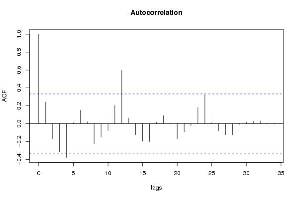
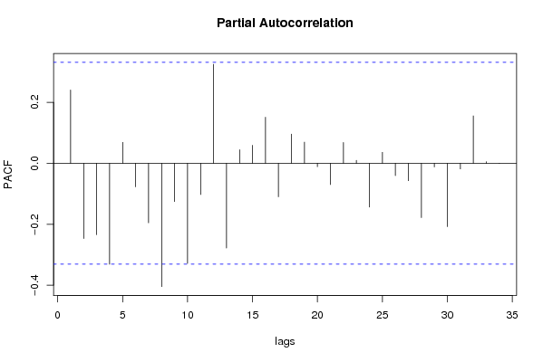
Title produced by software

(Partial) Autocorrelation Function

Date of computation

Mon, 22 Dec 2008 05:23:56 -0700

Cite this page as follows

Statistical Computations at FreeStatistics.org, Office for Research Development and Education, URL https://freestatistics.org/blog/index.php?v=date/2008/Dec/22/t12299486835xbfirgaasfcb55.htm/, Retrieved Sun, 12 May 2024 13:35:41 +0000

Statistical Computations at FreeStatistics.org, Office for Research Development and Education, URL https://freestatistics.org/blog/index.php?pk=36019, Retrieved Sun, 12 May 2024 13:35:41 +0000

QR Codes:

Paste this QR Code to cite your computation.

Original text written by user:

IsPrivate?

No (this computation is public)

User-defined keywords

Estimated Impact

184

Family? (F = Feedback message, R = changed R code, M = changed R Module, P = changed Parameters, D = changed Data)

-     [(Partial) Autocorrelation Function] [(P)ACF werkloosheid] [2008-12-21 22:54:14] [7a4703cb85a198d9845d72899eff0288]
-   P   [(Partial) Autocorrelation Function] [(P)ACF werkloosheid] [2008-12-21 23:29:15] [7a4703cb85a198d9845d72899eff0288]
-   P       [(Partial) Autocorrelation Function] [(P)ACF werklooshe...] [2008-12-22 12:23:56] [9f72e095d5529918bf5b0810c01bf6ce] [Current]
-   P         [(Partial) Autocorrelation Function] [(P)ACF Werklooshe...] [2008-12-22 12:31:57] [7a4703cb85a198d9845d72899eff0288] 
- RMP         [Spectral Analysis] [Spectral analysis...] [2008-12-22 12:38:27] [7a4703cb85a198d9845d72899eff0288] 
-   P           [Spectral Analysis] [Spectral Analysis...] [2008-12-22 13:08:13] [7a4703cb85a198d9845d72899eff0288] 
-   P             [Spectral Analysis] [Spectral analysis...] [2008-12-22 13:40:53] [7a4703cb85a198d9845d72899eff0288] 
-   P               [Spectral Analysis] [Spectral Analysis...] [2008-12-22 13:59:31] [7a4703cb85a198d9845d72899eff0288] 
- RMP               [ARIMA Forecasting] [] [2008-12-22 19:20:32] [b98453cac15ba1066b407e146608df68] 
- RMPD          [ARIMA Backward Selection] [ARIMA Backward Se...] [2008-12-23 13:32:19] [7a4703cb85a198d9845d72899eff0288] 

Feedback Forum

Post a new message

Dataseries X:

Download CSV

Histogram

Boxplots

Summary of computational transaction
Raw Input	view raw input (R code)
Raw Output	view raw output of R engine
Computing time	1 seconds
R Server	'George Udny Yule' @ 72.249.76.132

\begin{tabular}{lllllllll}
\hline
Summary of computational transaction \tabularnewline
Raw Input & view raw input (R code)  \tabularnewline
Raw Output & view raw output of R engine  \tabularnewline
Computing time & 1 seconds \tabularnewline
R Server & 'George Udny Yule' @ 72.249.76.132 \tabularnewline
\hline
\end{tabular}
%Source: https://freestatistics.org/blog/index.php?pk=36019&T=0

[TABLE]
[ROW][C]Summary of computational transaction[/C][/ROW]
[ROW][C]Raw Input[/C][C]view raw input (R code) [/C][/ROW]
[ROW][C]Raw Output[/C][C]view raw output of R engine [/C][/ROW]
[ROW][C]Computing time[/C][C]1 seconds[/C][/ROW]
[ROW][C]R Server[/C][C]'George Udny Yule' @ 72.249.76.132[/C][/ROW]
[/TABLE]
Source: https://freestatistics.org/blog/index.php?pk=36019&T=0

Globally Unique Identifier (entire table): ba.freestatistics.org/blog/index.php?pk=36019&T=0

As an alternative you can also use a QR Code:

The GUIDs for individual cells are displayed in the table below:

Summary of computational transaction
Raw Input	view raw input (R code)
Raw Output	view raw output of R engine
Computing time	1 seconds
R Server	'George Udny Yule' @ 72.249.76.132

Autocorrelation Function
Time lag k	ACF(k)	T-STAT	P-value
1	0.240723	1.4241	0.081631
2	-0.174643	-1.0332	0.154298
3	-0.319123	-1.888	0.033672
4	-0.379856	-2.2473	0.015515
5	0.010845	0.0642	0.474603
6	0.15038	0.8897	0.189861
7	0.020693	0.1224	0.451632
8	-0.223878	-1.3245	0.096964
9	-0.150695	-0.8915	0.189368
10	-0.079764	-0.4719	0.319967
11	0.205528	1.2159	0.116077
12	0.595717	3.5243	0.000602
13	0.061503	0.3639	0.359077
14	-0.123971	-0.7334	0.234092
15	-0.196042	-1.1598	0.126991
16	-0.199926	-1.1828	0.122435
17	0.016307	0.0965	0.461847
18	0.088038	0.5208	0.302879
19	-0.004082	-0.0241	0.490435
20	-0.171883	-1.0169	0.158096
21	-0.093591	-0.5537	0.291654
22	-0.023746	-0.1405	0.444542
23	0.180814	1.0697	0.146037
24	0.323683	1.9149	0.031851
25	0.009082	0.0537	0.478728
26	-0.084496	-0.4999	0.310142
27	-0.126418	-0.7479	0.229758
28	-0.126484	-0.7483	0.229641
29	-0.005666	-0.0335	0.486724
30	0.018912	0.1119	0.455778
31	0.027412	0.1622	0.436051
32	0.029934	0.1771	0.430228
33	0.008559	0.0506	0.479951
34	-0.003866	-0.0229	0.490942
35	NA	NA	NA
36	NA	NA	NA

\begin{tabular}{lllllllll}
\hline
Autocorrelation Function \tabularnewline
Time lag k & ACF(k) & T-STAT & P-value \tabularnewline
1 & 0.240723 & 1.4241 & 0.081631 \tabularnewline
2 & -0.174643 & -1.0332 & 0.154298 \tabularnewline
3 & -0.319123 & -1.888 & 0.033672 \tabularnewline
4 & -0.379856 & -2.2473 & 0.015515 \tabularnewline
5 & 0.010845 & 0.0642 & 0.474603 \tabularnewline
6 & 0.15038 & 0.8897 & 0.189861 \tabularnewline
7 & 0.020693 & 0.1224 & 0.451632 \tabularnewline
8 & -0.223878 & -1.3245 & 0.096964 \tabularnewline
9 & -0.150695 & -0.8915 & 0.189368 \tabularnewline
10 & -0.079764 & -0.4719 & 0.319967 \tabularnewline
11 & 0.205528 & 1.2159 & 0.116077 \tabularnewline
12 & 0.595717 & 3.5243 & 0.000602 \tabularnewline
13 & 0.061503 & 0.3639 & 0.359077 \tabularnewline
14 & -0.123971 & -0.7334 & 0.234092 \tabularnewline
15 & -0.196042 & -1.1598 & 0.126991 \tabularnewline
16 & -0.199926 & -1.1828 & 0.122435 \tabularnewline
17 & 0.016307 & 0.0965 & 0.461847 \tabularnewline
18 & 0.088038 & 0.5208 & 0.302879 \tabularnewline
19 & -0.004082 & -0.0241 & 0.490435 \tabularnewline
20 & -0.171883 & -1.0169 & 0.158096 \tabularnewline
21 & -0.093591 & -0.5537 & 0.291654 \tabularnewline
22 & -0.023746 & -0.1405 & 0.444542 \tabularnewline
23 & 0.180814 & 1.0697 & 0.146037 \tabularnewline
24 & 0.323683 & 1.9149 & 0.031851 \tabularnewline
25 & 0.009082 & 0.0537 & 0.478728 \tabularnewline
26 & -0.084496 & -0.4999 & 0.310142 \tabularnewline
27 & -0.126418 & -0.7479 & 0.229758 \tabularnewline
28 & -0.126484 & -0.7483 & 0.229641 \tabularnewline
29 & -0.005666 & -0.0335 & 0.486724 \tabularnewline
30 & 0.018912 & 0.1119 & 0.455778 \tabularnewline
31 & 0.027412 & 0.1622 & 0.436051 \tabularnewline
32 & 0.029934 & 0.1771 & 0.430228 \tabularnewline
33 & 0.008559 & 0.0506 & 0.479951 \tabularnewline
34 & -0.003866 & -0.0229 & 0.490942 \tabularnewline
35 & NA & NA & NA \tabularnewline
36 & NA & NA & NA \tabularnewline
\hline
\end{tabular}
%Source: https://freestatistics.org/blog/index.php?pk=36019&T=1

[TABLE]
[ROW][C]Autocorrelation Function[/C][/ROW]
[ROW][C]Time lag k[/C][C]ACF(k)[/C][C]T-STAT[/C][C]P-value[/C][/ROW]
[ROW][C]1[/C][C]0.240723[/C][C]1.4241[/C][C]0.081631[/C][/ROW]
[ROW][C]2[/C][C]-0.174643[/C][C]-1.0332[/C][C]0.154298[/C][/ROW]
[ROW][C]3[/C][C]-0.319123[/C][C]-1.888[/C][C]0.033672[/C][/ROW]
[ROW][C]4[/C][C]-0.379856[/C][C]-2.2473[/C][C]0.015515[/C][/ROW]
[ROW][C]5[/C][C]0.010845[/C][C]0.0642[/C][C]0.474603[/C][/ROW]
[ROW][C]6[/C][C]0.15038[/C][C]0.8897[/C][C]0.189861[/C][/ROW]
[ROW][C]7[/C][C]0.020693[/C][C]0.1224[/C][C]0.451632[/C][/ROW]
[ROW][C]8[/C][C]-0.223878[/C][C]-1.3245[/C][C]0.096964[/C][/ROW]
[ROW][C]9[/C][C]-0.150695[/C][C]-0.8915[/C][C]0.189368[/C][/ROW]
[ROW][C]10[/C][C]-0.079764[/C][C]-0.4719[/C][C]0.319967[/C][/ROW]
[ROW][C]11[/C][C]0.205528[/C][C]1.2159[/C][C]0.116077[/C][/ROW]
[ROW][C]12[/C][C]0.595717[/C][C]3.5243[/C][C]0.000602[/C][/ROW]
[ROW][C]13[/C][C]0.061503[/C][C]0.3639[/C][C]0.359077[/C][/ROW]
[ROW][C]14[/C][C]-0.123971[/C][C]-0.7334[/C][C]0.234092[/C][/ROW]
[ROW][C]15[/C][C]-0.196042[/C][C]-1.1598[/C][C]0.126991[/C][/ROW]
[ROW][C]16[/C][C]-0.199926[/C][C]-1.1828[/C][C]0.122435[/C][/ROW]
[ROW][C]17[/C][C]0.016307[/C][C]0.0965[/C][C]0.461847[/C][/ROW]
[ROW][C]18[/C][C]0.088038[/C][C]0.5208[/C][C]0.302879[/C][/ROW]
[ROW][C]19[/C][C]-0.004082[/C][C]-0.0241[/C][C]0.490435[/C][/ROW]
[ROW][C]20[/C][C]-0.171883[/C][C]-1.0169[/C][C]0.158096[/C][/ROW]
[ROW][C]21[/C][C]-0.093591[/C][C]-0.5537[/C][C]0.291654[/C][/ROW]
[ROW][C]22[/C][C]-0.023746[/C][C]-0.1405[/C][C]0.444542[/C][/ROW]
[ROW][C]23[/C][C]0.180814[/C][C]1.0697[/C][C]0.146037[/C][/ROW]
[ROW][C]24[/C][C]0.323683[/C][C]1.9149[/C][C]0.031851[/C][/ROW]
[ROW][C]25[/C][C]0.009082[/C][C]0.0537[/C][C]0.478728[/C][/ROW]
[ROW][C]26[/C][C]-0.084496[/C][C]-0.4999[/C][C]0.310142[/C][/ROW]
[ROW][C]27[/C][C]-0.126418[/C][C]-0.7479[/C][C]0.229758[/C][/ROW]
[ROW][C]28[/C][C]-0.126484[/C][C]-0.7483[/C][C]0.229641[/C][/ROW]
[ROW][C]29[/C][C]-0.005666[/C][C]-0.0335[/C][C]0.486724[/C][/ROW]
[ROW][C]30[/C][C]0.018912[/C][C]0.1119[/C][C]0.455778[/C][/ROW]
[ROW][C]31[/C][C]0.027412[/C][C]0.1622[/C][C]0.436051[/C][/ROW]
[ROW][C]32[/C][C]0.029934[/C][C]0.1771[/C][C]0.430228[/C][/ROW]
[ROW][C]33[/C][C]0.008559[/C][C]0.0506[/C][C]0.479951[/C][/ROW]
[ROW][C]34[/C][C]-0.003866[/C][C]-0.0229[/C][C]0.490942[/C][/ROW]
[ROW][C]35[/C][C]NA[/C][C]NA[/C][C]NA[/C][/ROW]
[ROW][C]36[/C][C]NA[/C][C]NA[/C][C]NA[/C][/ROW]
[/TABLE]
Source: https://freestatistics.org/blog/index.php?pk=36019&T=1

Globally Unique Identifier (entire table): ba.freestatistics.org/blog/index.php?pk=36019&T=1

As an alternative you can also use a QR Code:

The GUIDs for individual cells are displayed in the table below:

Autocorrelation Function
Time lag k	ACF(k)	T-STAT	P-value
1	0.240723	1.4241	0.081631
2	-0.174643	-1.0332	0.154298
3	-0.319123	-1.888	0.033672
4	-0.379856	-2.2473	0.015515
5	0.010845	0.0642	0.474603
6	0.15038	0.8897	0.189861
7	0.020693	0.1224	0.451632
8	-0.223878	-1.3245	0.096964
9	-0.150695	-0.8915	0.189368
10	-0.079764	-0.4719	0.319967
11	0.205528	1.2159	0.116077
12	0.595717	3.5243	0.000602
13	0.061503	0.3639	0.359077
14	-0.123971	-0.7334	0.234092
15	-0.196042	-1.1598	0.126991
16	-0.199926	-1.1828	0.122435
17	0.016307	0.0965	0.461847
18	0.088038	0.5208	0.302879
19	-0.004082	-0.0241	0.490435
20	-0.171883	-1.0169	0.158096
21	-0.093591	-0.5537	0.291654
22	-0.023746	-0.1405	0.444542
23	0.180814	1.0697	0.146037
24	0.323683	1.9149	0.031851
25	0.009082	0.0537	0.478728
26	-0.084496	-0.4999	0.310142
27	-0.126418	-0.7479	0.229758
28	-0.126484	-0.7483	0.229641
29	-0.005666	-0.0335	0.486724
30	0.018912	0.1119	0.455778
31	0.027412	0.1622	0.436051
32	0.029934	0.1771	0.430228
33	0.008559	0.0506	0.479951
34	-0.003866	-0.0229	0.490942
35	NA	NA	NA
36	NA	NA	NA

Partial Autocorrelation Function
Time lag k	PACF(k)	T-STAT	P-value
1	0.240723	1.4241	0.081631
2	-0.246898	-1.4607	0.076513
3	-0.234301	-1.3861	0.087236
4	-0.331274	-1.9598	0.029008
5	0.068835	0.4072	0.343159
6	-0.077367	-0.4577	0.324995
7	-0.195142	-1.1545	0.128064
8	-0.404673	-2.3941	0.011077
9	-0.125501	-0.7425	0.231378
10	-0.328728	-1.9448	0.029936
11	-0.102604	-0.607	0.273879
12	0.32511	1.9234	0.031299
13	-0.278113	-1.6453	0.054427
14	0.044697	0.2644	0.3965
15	0.05908	0.3495	0.364396
16	0.151224	0.8947	0.188542
17	-0.109976	-0.6506	0.259768
18	0.09592	0.5675	0.287008
19	0.069509	0.4112	0.34171
20	-0.011245	-0.0665	0.473669
21	-0.069803	-0.413	0.341076
22	0.068389	0.4046	0.344119
23	0.009533	0.0564	0.477672
24	-0.143806	-0.8508	0.20034
25	0.036085	0.2135	0.416094
26	-0.040625	-0.2403	0.405733
27	-0.057134	-0.338	0.368687
28	-0.178299	-1.0548	0.149365
29	-0.01186	-0.0702	0.472231
30	-0.207806	-1.2294	0.113562
31	-0.018535	-0.1097	0.456656
32	0.155519	0.9201	0.181919
33	0.005322	0.0315	0.487531
34	0.000605	0.0036	0.498583
35	NA	NA	NA
36	NA	NA	NA

\begin{tabular}{lllllllll}
\hline
Partial Autocorrelation Function \tabularnewline
Time lag k & PACF(k) & T-STAT & P-value \tabularnewline
1 & 0.240723 & 1.4241 & 0.081631 \tabularnewline
2 & -0.246898 & -1.4607 & 0.076513 \tabularnewline
3 & -0.234301 & -1.3861 & 0.087236 \tabularnewline
4 & -0.331274 & -1.9598 & 0.029008 \tabularnewline
5 & 0.068835 & 0.4072 & 0.343159 \tabularnewline
6 & -0.077367 & -0.4577 & 0.324995 \tabularnewline
7 & -0.195142 & -1.1545 & 0.128064 \tabularnewline
8 & -0.404673 & -2.3941 & 0.011077 \tabularnewline
9 & -0.125501 & -0.7425 & 0.231378 \tabularnewline
10 & -0.328728 & -1.9448 & 0.029936 \tabularnewline
11 & -0.102604 & -0.607 & 0.273879 \tabularnewline
12 & 0.32511 & 1.9234 & 0.031299 \tabularnewline
13 & -0.278113 & -1.6453 & 0.054427 \tabularnewline
14 & 0.044697 & 0.2644 & 0.3965 \tabularnewline
15 & 0.05908 & 0.3495 & 0.364396 \tabularnewline
16 & 0.151224 & 0.8947 & 0.188542 \tabularnewline
17 & -0.109976 & -0.6506 & 0.259768 \tabularnewline
18 & 0.09592 & 0.5675 & 0.287008 \tabularnewline
19 & 0.069509 & 0.4112 & 0.34171 \tabularnewline
20 & -0.011245 & -0.0665 & 0.473669 \tabularnewline
21 & -0.069803 & -0.413 & 0.341076 \tabularnewline
22 & 0.068389 & 0.4046 & 0.344119 \tabularnewline
23 & 0.009533 & 0.0564 & 0.477672 \tabularnewline
24 & -0.143806 & -0.8508 & 0.20034 \tabularnewline
25 & 0.036085 & 0.2135 & 0.416094 \tabularnewline
26 & -0.040625 & -0.2403 & 0.405733 \tabularnewline
27 & -0.057134 & -0.338 & 0.368687 \tabularnewline
28 & -0.178299 & -1.0548 & 0.149365 \tabularnewline
29 & -0.01186 & -0.0702 & 0.472231 \tabularnewline
30 & -0.207806 & -1.2294 & 0.113562 \tabularnewline
31 & -0.018535 & -0.1097 & 0.456656 \tabularnewline
32 & 0.155519 & 0.9201 & 0.181919 \tabularnewline
33 & 0.005322 & 0.0315 & 0.487531 \tabularnewline
34 & 0.000605 & 0.0036 & 0.498583 \tabularnewline
35 & NA & NA & NA \tabularnewline
36 & NA & NA & NA \tabularnewline
\hline
\end{tabular}
%Source: https://freestatistics.org/blog/index.php?pk=36019&T=2

[TABLE]
[ROW][C]Partial Autocorrelation Function[/C][/ROW]
[ROW][C]Time lag k[/C][C]PACF(k)[/C][C]T-STAT[/C][C]P-value[/C][/ROW]
[ROW][C]1[/C][C]0.240723[/C][C]1.4241[/C][C]0.081631[/C][/ROW]
[ROW][C]2[/C][C]-0.246898[/C][C]-1.4607[/C][C]0.076513[/C][/ROW]
[ROW][C]3[/C][C]-0.234301[/C][C]-1.3861[/C][C]0.087236[/C][/ROW]
[ROW][C]4[/C][C]-0.331274[/C][C]-1.9598[/C][C]0.029008[/C][/ROW]
[ROW][C]5[/C][C]0.068835[/C][C]0.4072[/C][C]0.343159[/C][/ROW]
[ROW][C]6[/C][C]-0.077367[/C][C]-0.4577[/C][C]0.324995[/C][/ROW]
[ROW][C]7[/C][C]-0.195142[/C][C]-1.1545[/C][C]0.128064[/C][/ROW]
[ROW][C]8[/C][C]-0.404673[/C][C]-2.3941[/C][C]0.011077[/C][/ROW]
[ROW][C]9[/C][C]-0.125501[/C][C]-0.7425[/C][C]0.231378[/C][/ROW]
[ROW][C]10[/C][C]-0.328728[/C][C]-1.9448[/C][C]0.029936[/C][/ROW]
[ROW][C]11[/C][C]-0.102604[/C][C]-0.607[/C][C]0.273879[/C][/ROW]
[ROW][C]12[/C][C]0.32511[/C][C]1.9234[/C][C]0.031299[/C][/ROW]
[ROW][C]13[/C][C]-0.278113[/C][C]-1.6453[/C][C]0.054427[/C][/ROW]
[ROW][C]14[/C][C]0.044697[/C][C]0.2644[/C][C]0.3965[/C][/ROW]
[ROW][C]15[/C][C]0.05908[/C][C]0.3495[/C][C]0.364396[/C][/ROW]
[ROW][C]16[/C][C]0.151224[/C][C]0.8947[/C][C]0.188542[/C][/ROW]
[ROW][C]17[/C][C]-0.109976[/C][C]-0.6506[/C][C]0.259768[/C][/ROW]
[ROW][C]18[/C][C]0.09592[/C][C]0.5675[/C][C]0.287008[/C][/ROW]
[ROW][C]19[/C][C]0.069509[/C][C]0.4112[/C][C]0.34171[/C][/ROW]
[ROW][C]20[/C][C]-0.011245[/C][C]-0.0665[/C][C]0.473669[/C][/ROW]
[ROW][C]21[/C][C]-0.069803[/C][C]-0.413[/C][C]0.341076[/C][/ROW]
[ROW][C]22[/C][C]0.068389[/C][C]0.4046[/C][C]0.344119[/C][/ROW]
[ROW][C]23[/C][C]0.009533[/C][C]0.0564[/C][C]0.477672[/C][/ROW]
[ROW][C]24[/C][C]-0.143806[/C][C]-0.8508[/C][C]0.20034[/C][/ROW]
[ROW][C]25[/C][C]0.036085[/C][C]0.2135[/C][C]0.416094[/C][/ROW]
[ROW][C]26[/C][C]-0.040625[/C][C]-0.2403[/C][C]0.405733[/C][/ROW]
[ROW][C]27[/C][C]-0.057134[/C][C]-0.338[/C][C]0.368687[/C][/ROW]
[ROW][C]28[/C][C]-0.178299[/C][C]-1.0548[/C][C]0.149365[/C][/ROW]
[ROW][C]29[/C][C]-0.01186[/C][C]-0.0702[/C][C]0.472231[/C][/ROW]
[ROW][C]30[/C][C]-0.207806[/C][C]-1.2294[/C][C]0.113562[/C][/ROW]
[ROW][C]31[/C][C]-0.018535[/C][C]-0.1097[/C][C]0.456656[/C][/ROW]
[ROW][C]32[/C][C]0.155519[/C][C]0.9201[/C][C]0.181919[/C][/ROW]
[ROW][C]33[/C][C]0.005322[/C][C]0.0315[/C][C]0.487531[/C][/ROW]
[ROW][C]34[/C][C]0.000605[/C][C]0.0036[/C][C]0.498583[/C][/ROW]
[ROW][C]35[/C][C]NA[/C][C]NA[/C][C]NA[/C][/ROW]
[ROW][C]36[/C][C]NA[/C][C]NA[/C][C]NA[/C][/ROW]
[/TABLE]
Source: https://freestatistics.org/blog/index.php?pk=36019&T=2

Globally Unique Identifier (entire table): ba.freestatistics.org/blog/index.php?pk=36019&T=2

As an alternative you can also use a QR Code:

The GUIDs for individual cells are displayed in the table below:

Partial Autocorrelation Function
Time lag k	PACF(k)	T-STAT	P-value
1	0.240723	1.4241	0.081631
2	-0.246898	-1.4607	0.076513
3	-0.234301	-1.3861	0.087236
4	-0.331274	-1.9598	0.029008
5	0.068835	0.4072	0.343159
6	-0.077367	-0.4577	0.324995
7	-0.195142	-1.1545	0.128064
8	-0.404673	-2.3941	0.011077
9	-0.125501	-0.7425	0.231378
10	-0.328728	-1.9448	0.029936
11	-0.102604	-0.607	0.273879
12	0.32511	1.9234	0.031299
13	-0.278113	-1.6453	0.054427
14	0.044697	0.2644	0.3965
15	0.05908	0.3495	0.364396
16	0.151224	0.8947	0.188542
17	-0.109976	-0.6506	0.259768
18	0.09592	0.5675	0.287008
19	0.069509	0.4112	0.34171
20	-0.011245	-0.0665	0.473669
21	-0.069803	-0.413	0.341076
22	0.068389	0.4046	0.344119
23	0.009533	0.0564	0.477672
24	-0.143806	-0.8508	0.20034
25	0.036085	0.2135	0.416094
26	-0.040625	-0.2403	0.405733
27	-0.057134	-0.338	0.368687
28	-0.178299	-1.0548	0.149365
29	-0.01186	-0.0702	0.472231
30	-0.207806	-1.2294	0.113562
31	-0.018535	-0.1097	0.456656
32	0.155519	0.9201	0.181919
33	0.005322	0.0315	0.487531
34	0.000605	0.0036	0.498583
35	NA	NA	NA
36	NA	NA	NA

Figure 1

PNG link

Postscript link

PDF link

Figure 2

PNG link

Postscript link

PDF link

Parameters (Session):

par1 = 36 ; par2 = 1 ; par3 = 1 ; par4 = 0 ; par5 = 12 ;

Parameters (R input):

par1 = 36 ; par2 = 1 ; par3 = 1 ; par4 = 0 ; par5 = 12 ;

R code (references can be found in the software module):

if (par1 == 'Default') {
par1 = 10*log10(length(x))
} else {
par1 <- as.numeric(par1)
}
par2 <- as.numeric(par2)
par3 <- as.numeric(par3)
par4 <- as.numeric(par4)
par5 <- as.numeric(par5)
if (par2 == 0) {
x <- log(x)
} else {
x <- (x ^ par2 - 1) / par2
}
if (par3 > 0) x <- diff(x,lag=1,difference=par3)
if (par4 > 0) x <- diff(x,lag=par5,difference=par4)
bitmap(file='pic1.png')
racf <- acf(x,par1,main='Autocorrelation',xlab='lags',ylab='ACF')
dev.off()
bitmap(file='pic2.png')
rpacf <- pacf(x,par1,main='Partial Autocorrelation',xlab='lags',ylab='PACF')
dev.off()
(myacf <- c(racf$acf))
(mypacf <- c(rpacf$acf))
lengthx <- length(x)
sqrtn <- sqrt(lengthx)
load(file='createtable')
a<-table.start()
a<-table.row.start(a)
a<-table.element(a,'Autocorrelation Function',4,TRUE)
a<-table.row.end(a)
a<-table.row.start(a)
a<-table.element(a,'Time lag k',header=TRUE)
a<-table.element(a,hyperlink('basics.htm','ACF(k)','click here for more information about the Autocorrelation Function'),header=TRUE)
a<-table.element(a,'T-STAT',header=TRUE)
a<-table.element(a,'P-value',header=TRUE)
a<-table.row.end(a)
for (i in 2:(par1+1)) {
a<-table.row.start(a)
a<-table.element(a,i-1,header=TRUE)
a<-table.element(a,round(myacf[i],6))
mytstat <- myacf[i]*sqrtn
a<-table.element(a,round(mytstat,4))
a<-table.element(a,round(1-pt(abs(mytstat),lengthx),6))
a<-table.row.end(a)
}
a<-table.end(a)
table.save(a,file='mytable.tab')
a<-table.start()
a<-table.row.start(a)
a<-table.element(a,'Partial Autocorrelation Function',4,TRUE)
a<-table.row.end(a)
a<-table.row.start(a)
a<-table.element(a,'Time lag k',header=TRUE)
a<-table.element(a,hyperlink('basics.htm','PACF(k)','click here for more information about the Partial Autocorrelation Function'),header=TRUE)
a<-table.element(a,'T-STAT',header=TRUE)
a<-table.element(a,'P-value',header=TRUE)
a<-table.row.end(a)
for (i in 1:par1) {
a<-table.row.start(a)
a<-table.element(a,i,header=TRUE)
a<-table.element(a,round(mypacf[i],6))
mytstat <- mypacf[i]*sqrtn
a<-table.element(a,round(mytstat,4))
a<-table.element(a,round(1-pt(abs(mytstat),lengthx),6))
a<-table.row.end(a)
}
a<-table.end(a)
table.save(a,file='mytable1.tab')

Free Statistics

Description of Statistical Computation

Tree of Dependent Computations

Dataset

Tables (Output of Computation)

Figures (Output of Computation)

Input Parameters & R Code