Repository of Reproducible Computations

Free Statistics

of Irreproducible Research!

Author's title

Author

*The author of this computation has been verified*

R Software Module

rwasp_autocorrelation.wasp

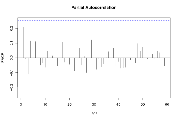
Title produced by software

(Partial) Autocorrelation Function

Date of computation

Mon, 22 Dec 2008 01:38:52 -0700

Cite this page as follows

Statistical Computations at FreeStatistics.org, Office for Research Development and Education, URL https://freestatistics.org/blog/index.php?v=date/2008/Dec/22/t1229942090jdz0akzwk3493st.htm/, Retrieved Mon, 13 May 2024 03:25:44 +0000

Statistical Computations at FreeStatistics.org, Office for Research Development and Education, URL https://freestatistics.org/blog/index.php?pk=35988, Retrieved Mon, 13 May 2024 03:25:44 +0000

QR Codes:

Paste this QR Code to cite your computation.

Original text written by user:

IsPrivate?

No (this computation is public)

User-defined keywords

Estimated Impact

182

Family? (F = Feedback message, R = changed R code, M = changed R Module, P = changed Parameters, D = changed Data)

F     [Univariate Data Series] [blog 1e tijdreeks...] [2008-10-13 19:23:31] [7173087adebe3e3a714c80ea2417b3eb]
-   PD  [Univariate Data Series] [tijdreeksen opnie...] [2008-10-19 17:13:12] [7173087adebe3e3a714c80ea2417b3eb]
-   PD    [Univariate Data Series] [tijdreeksen opnie...] [2008-10-19 18:55:20] [7173087adebe3e3a714c80ea2417b3eb]
- RM        [Central Tendency] [central tendency ...] [2008-10-19 19:10:37] [7173087adebe3e3a714c80ea2417b3eb]
- RMP         [(Partial) Autocorrelation Function] [ACF step 2 own da...] [2008-12-08 20:48:28] [7173087adebe3e3a714c80ea2417b3eb]
-   PD            [(Partial) Autocorrelation Function] [] [2008-12-22 08:38:52] [0e4dd4b7713a9edf1ca3fab1bbbafcc9] [Current]

Feedback Forum

Post a new message

Dataseries X:

Download CSV

Histogram

Boxplots

Summary of computational transaction
Raw Input	view raw input (R code)
Raw Output	view raw output of R engine
Computing time	1 seconds
R Server	'Gwilym Jenkins' @ 72.249.127.135

\begin{tabular}{lllllllll}
\hline
Summary of computational transaction \tabularnewline
Raw Input & view raw input (R code)  \tabularnewline
Raw Output & view raw output of R engine  \tabularnewline
Computing time & 1 seconds \tabularnewline
R Server & 'Gwilym Jenkins' @ 72.249.127.135 \tabularnewline
\hline
\end{tabular}
%Source: https://freestatistics.org/blog/index.php?pk=35988&T=0

[TABLE]
[ROW][C]Summary of computational transaction[/C][/ROW]
[ROW][C]Raw Input[/C][C]view raw input (R code) [/C][/ROW]
[ROW][C]Raw Output[/C][C]view raw output of R engine [/C][/ROW]
[ROW][C]Computing time[/C][C]1 seconds[/C][/ROW]
[ROW][C]R Server[/C][C]'Gwilym Jenkins' @ 72.249.127.135[/C][/ROW]
[/TABLE]
Source: https://freestatistics.org/blog/index.php?pk=35988&T=0

Globally Unique Identifier (entire table): ba.freestatistics.org/blog/index.php?pk=35988&T=0

As an alternative you can also use a QR Code:

The GUIDs for individual cells are displayed in the table below:

Summary of computational transaction
Raw Input	view raw input (R code)
Raw Output	view raw output of R engine
Computing time	1 seconds
R Server	'Gwilym Jenkins' @ 72.249.127.135

Autocorrelation Function
Time lag k	ACF(k)	T-STAT	P-value
1	0.20759	1.608	0.056544
2	0.03541	0.2743	0.392403
3	-0.100439	-0.778	0.219813
4	0.065919	0.5106	0.30575
5	0.161376	1.25	0.108074
6	0.181982	1.4096	0.081906
7	0.101557	0.7867	0.21729
8	-0.033525	-0.2597	0.397999
9	-0.051962	-0.4025	0.344374
10	-0.053204	-0.4121	0.340861
11	0.078042	0.6045	0.273891
12	0.177832	1.3775	0.08674
13	0.086464	0.6697	0.252793
14	0.005903	0.0457	0.481841
15	-0.092287	-0.7149	0.238735
16	-0.033434	-0.259	0.398269
17	0.131605	1.0194	0.156051
18	0.088763	0.6876	0.247192
19	-0.022474	-0.1741	0.431195
20	-0.100009	-0.7747	0.220789
21	-0.105315	-0.8158	0.20893
22	-0.103034	-0.7981	0.213981
23	0.031503	0.244	0.404022
24	0.093135	0.7214	0.236726
25	-0.020126	-0.1559	0.438321
26	-0.057261	-0.4435	0.329485
27	-0.180451	-1.3978	0.083664
28	-0.119788	-0.9279	0.178595
29	0.105592	0.8179	0.208323
30	-0.012843	-0.0995	0.460544
31	-0.08119	-0.6289	0.265902
32	-0.149628	-1.159	0.125521
33	-0.143246	-1.1096	0.135804
34	-0.100077	-0.7752	0.220636
35	-0.00223	-0.0173	0.493138
36	0.036972	0.2864	0.387784
37	-0.032672	-0.2531	0.400538
38	-0.01186	-0.0919	0.463554
39	-0.152323	-1.1799	0.12135
40	-0.061758	-0.4784	0.317061
41	-0.038054	-0.2948	0.384594
42	-0.023875	-0.1849	0.426951
43	-0.06818	-0.5281	0.299681
44	-0.151422	-1.1729	0.122734
45	-0.135211	-1.0473	0.149571
46	-0.06978	-0.5405	0.295421
47	-0.025574	-0.1981	0.42182
48	0.0361	0.2796	0.390363
49	0.032171	0.2492	0.402032
50	0.045537	0.3527	0.362763
51	-0.10299	-0.7978	0.214078
52	-0.004048	-0.0314	0.487545
53	0.109122	0.8453	0.200663
54	0.114734	0.8887	0.18885
55	0.074255	0.5752	0.283662
56	-0.019598	-0.1518	0.439924
57	-0.024599	-0.1905	0.424764
58	-0.015704	-0.1216	0.451795
59	-0.001391	-0.0108	0.495718
60	NA	NA	NA

\begin{tabular}{lllllllll}
\hline
Autocorrelation Function \tabularnewline
Time lag k & ACF(k) & T-STAT & P-value \tabularnewline
1 & 0.20759 & 1.608 & 0.056544 \tabularnewline
2 & 0.03541 & 0.2743 & 0.392403 \tabularnewline
3 & -0.100439 & -0.778 & 0.219813 \tabularnewline
4 & 0.065919 & 0.5106 & 0.30575 \tabularnewline
5 & 0.161376 & 1.25 & 0.108074 \tabularnewline
6 & 0.181982 & 1.4096 & 0.081906 \tabularnewline
7 & 0.101557 & 0.7867 & 0.21729 \tabularnewline
8 & -0.033525 & -0.2597 & 0.397999 \tabularnewline
9 & -0.051962 & -0.4025 & 0.344374 \tabularnewline
10 & -0.053204 & -0.4121 & 0.340861 \tabularnewline
11 & 0.078042 & 0.6045 & 0.273891 \tabularnewline
12 & 0.177832 & 1.3775 & 0.08674 \tabularnewline
13 & 0.086464 & 0.6697 & 0.252793 \tabularnewline
14 & 0.005903 & 0.0457 & 0.481841 \tabularnewline
15 & -0.092287 & -0.7149 & 0.238735 \tabularnewline
16 & -0.033434 & -0.259 & 0.398269 \tabularnewline
17 & 0.131605 & 1.0194 & 0.156051 \tabularnewline
18 & 0.088763 & 0.6876 & 0.247192 \tabularnewline
19 & -0.022474 & -0.1741 & 0.431195 \tabularnewline
20 & -0.100009 & -0.7747 & 0.220789 \tabularnewline
21 & -0.105315 & -0.8158 & 0.20893 \tabularnewline
22 & -0.103034 & -0.7981 & 0.213981 \tabularnewline
23 & 0.031503 & 0.244 & 0.404022 \tabularnewline
24 & 0.093135 & 0.7214 & 0.236726 \tabularnewline
25 & -0.020126 & -0.1559 & 0.438321 \tabularnewline
26 & -0.057261 & -0.4435 & 0.329485 \tabularnewline
27 & -0.180451 & -1.3978 & 0.083664 \tabularnewline
28 & -0.119788 & -0.9279 & 0.178595 \tabularnewline
29 & 0.105592 & 0.8179 & 0.208323 \tabularnewline
30 & -0.012843 & -0.0995 & 0.460544 \tabularnewline
31 & -0.08119 & -0.6289 & 0.265902 \tabularnewline
32 & -0.149628 & -1.159 & 0.125521 \tabularnewline
33 & -0.143246 & -1.1096 & 0.135804 \tabularnewline
34 & -0.100077 & -0.7752 & 0.220636 \tabularnewline
35 & -0.00223 & -0.0173 & 0.493138 \tabularnewline
36 & 0.036972 & 0.2864 & 0.387784 \tabularnewline
37 & -0.032672 & -0.2531 & 0.400538 \tabularnewline
38 & -0.01186 & -0.0919 & 0.463554 \tabularnewline
39 & -0.152323 & -1.1799 & 0.12135 \tabularnewline
40 & -0.061758 & -0.4784 & 0.317061 \tabularnewline
41 & -0.038054 & -0.2948 & 0.384594 \tabularnewline
42 & -0.023875 & -0.1849 & 0.426951 \tabularnewline
43 & -0.06818 & -0.5281 & 0.299681 \tabularnewline
44 & -0.151422 & -1.1729 & 0.122734 \tabularnewline
45 & -0.135211 & -1.0473 & 0.149571 \tabularnewline
46 & -0.06978 & -0.5405 & 0.295421 \tabularnewline
47 & -0.025574 & -0.1981 & 0.42182 \tabularnewline
48 & 0.0361 & 0.2796 & 0.390363 \tabularnewline
49 & 0.032171 & 0.2492 & 0.402032 \tabularnewline
50 & 0.045537 & 0.3527 & 0.362763 \tabularnewline
51 & -0.10299 & -0.7978 & 0.214078 \tabularnewline
52 & -0.004048 & -0.0314 & 0.487545 \tabularnewline
53 & 0.109122 & 0.8453 & 0.200663 \tabularnewline
54 & 0.114734 & 0.8887 & 0.18885 \tabularnewline
55 & 0.074255 & 0.5752 & 0.283662 \tabularnewline
56 & -0.019598 & -0.1518 & 0.439924 \tabularnewline
57 & -0.024599 & -0.1905 & 0.424764 \tabularnewline
58 & -0.015704 & -0.1216 & 0.451795 \tabularnewline
59 & -0.001391 & -0.0108 & 0.495718 \tabularnewline
60 & NA & NA & NA \tabularnewline
\hline
\end{tabular}
%Source: https://freestatistics.org/blog/index.php?pk=35988&T=1

[TABLE]
[ROW][C]Autocorrelation Function[/C][/ROW]
[ROW][C]Time lag k[/C][C]ACF(k)[/C][C]T-STAT[/C][C]P-value[/C][/ROW]
[ROW][C]1[/C][C]0.20759[/C][C]1.608[/C][C]0.056544[/C][/ROW]
[ROW][C]2[/C][C]0.03541[/C][C]0.2743[/C][C]0.392403[/C][/ROW]
[ROW][C]3[/C][C]-0.100439[/C][C]-0.778[/C][C]0.219813[/C][/ROW]
[ROW][C]4[/C][C]0.065919[/C][C]0.5106[/C][C]0.30575[/C][/ROW]
[ROW][C]5[/C][C]0.161376[/C][C]1.25[/C][C]0.108074[/C][/ROW]
[ROW][C]6[/C][C]0.181982[/C][C]1.4096[/C][C]0.081906[/C][/ROW]
[ROW][C]7[/C][C]0.101557[/C][C]0.7867[/C][C]0.21729[/C][/ROW]
[ROW][C]8[/C][C]-0.033525[/C][C]-0.2597[/C][C]0.397999[/C][/ROW]
[ROW][C]9[/C][C]-0.051962[/C][C]-0.4025[/C][C]0.344374[/C][/ROW]
[ROW][C]10[/C][C]-0.053204[/C][C]-0.4121[/C][C]0.340861[/C][/ROW]
[ROW][C]11[/C][C]0.078042[/C][C]0.6045[/C][C]0.273891[/C][/ROW]
[ROW][C]12[/C][C]0.177832[/C][C]1.3775[/C][C]0.08674[/C][/ROW]
[ROW][C]13[/C][C]0.086464[/C][C]0.6697[/C][C]0.252793[/C][/ROW]
[ROW][C]14[/C][C]0.005903[/C][C]0.0457[/C][C]0.481841[/C][/ROW]
[ROW][C]15[/C][C]-0.092287[/C][C]-0.7149[/C][C]0.238735[/C][/ROW]
[ROW][C]16[/C][C]-0.033434[/C][C]-0.259[/C][C]0.398269[/C][/ROW]
[ROW][C]17[/C][C]0.131605[/C][C]1.0194[/C][C]0.156051[/C][/ROW]
[ROW][C]18[/C][C]0.088763[/C][C]0.6876[/C][C]0.247192[/C][/ROW]
[ROW][C]19[/C][C]-0.022474[/C][C]-0.1741[/C][C]0.431195[/C][/ROW]
[ROW][C]20[/C][C]-0.100009[/C][C]-0.7747[/C][C]0.220789[/C][/ROW]
[ROW][C]21[/C][C]-0.105315[/C][C]-0.8158[/C][C]0.20893[/C][/ROW]
[ROW][C]22[/C][C]-0.103034[/C][C]-0.7981[/C][C]0.213981[/C][/ROW]
[ROW][C]23[/C][C]0.031503[/C][C]0.244[/C][C]0.404022[/C][/ROW]
[ROW][C]24[/C][C]0.093135[/C][C]0.7214[/C][C]0.236726[/C][/ROW]
[ROW][C]25[/C][C]-0.020126[/C][C]-0.1559[/C][C]0.438321[/C][/ROW]
[ROW][C]26[/C][C]-0.057261[/C][C]-0.4435[/C][C]0.329485[/C][/ROW]
[ROW][C]27[/C][C]-0.180451[/C][C]-1.3978[/C][C]0.083664[/C][/ROW]
[ROW][C]28[/C][C]-0.119788[/C][C]-0.9279[/C][C]0.178595[/C][/ROW]
[ROW][C]29[/C][C]0.105592[/C][C]0.8179[/C][C]0.208323[/C][/ROW]
[ROW][C]30[/C][C]-0.012843[/C][C]-0.0995[/C][C]0.460544[/C][/ROW]
[ROW][C]31[/C][C]-0.08119[/C][C]-0.6289[/C][C]0.265902[/C][/ROW]
[ROW][C]32[/C][C]-0.149628[/C][C]-1.159[/C][C]0.125521[/C][/ROW]
[ROW][C]33[/C][C]-0.143246[/C][C]-1.1096[/C][C]0.135804[/C][/ROW]
[ROW][C]34[/C][C]-0.100077[/C][C]-0.7752[/C][C]0.220636[/C][/ROW]
[ROW][C]35[/C][C]-0.00223[/C][C]-0.0173[/C][C]0.493138[/C][/ROW]
[ROW][C]36[/C][C]0.036972[/C][C]0.2864[/C][C]0.387784[/C][/ROW]
[ROW][C]37[/C][C]-0.032672[/C][C]-0.2531[/C][C]0.400538[/C][/ROW]
[ROW][C]38[/C][C]-0.01186[/C][C]-0.0919[/C][C]0.463554[/C][/ROW]
[ROW][C]39[/C][C]-0.152323[/C][C]-1.1799[/C][C]0.12135[/C][/ROW]
[ROW][C]40[/C][C]-0.061758[/C][C]-0.4784[/C][C]0.317061[/C][/ROW]
[ROW][C]41[/C][C]-0.038054[/C][C]-0.2948[/C][C]0.384594[/C][/ROW]
[ROW][C]42[/C][C]-0.023875[/C][C]-0.1849[/C][C]0.426951[/C][/ROW]
[ROW][C]43[/C][C]-0.06818[/C][C]-0.5281[/C][C]0.299681[/C][/ROW]
[ROW][C]44[/C][C]-0.151422[/C][C]-1.1729[/C][C]0.122734[/C][/ROW]
[ROW][C]45[/C][C]-0.135211[/C][C]-1.0473[/C][C]0.149571[/C][/ROW]
[ROW][C]46[/C][C]-0.06978[/C][C]-0.5405[/C][C]0.295421[/C][/ROW]
[ROW][C]47[/C][C]-0.025574[/C][C]-0.1981[/C][C]0.42182[/C][/ROW]
[ROW][C]48[/C][C]0.0361[/C][C]0.2796[/C][C]0.390363[/C][/ROW]
[ROW][C]49[/C][C]0.032171[/C][C]0.2492[/C][C]0.402032[/C][/ROW]
[ROW][C]50[/C][C]0.045537[/C][C]0.3527[/C][C]0.362763[/C][/ROW]
[ROW][C]51[/C][C]-0.10299[/C][C]-0.7978[/C][C]0.214078[/C][/ROW]
[ROW][C]52[/C][C]-0.004048[/C][C]-0.0314[/C][C]0.487545[/C][/ROW]
[ROW][C]53[/C][C]0.109122[/C][C]0.8453[/C][C]0.200663[/C][/ROW]
[ROW][C]54[/C][C]0.114734[/C][C]0.8887[/C][C]0.18885[/C][/ROW]
[ROW][C]55[/C][C]0.074255[/C][C]0.5752[/C][C]0.283662[/C][/ROW]
[ROW][C]56[/C][C]-0.019598[/C][C]-0.1518[/C][C]0.439924[/C][/ROW]
[ROW][C]57[/C][C]-0.024599[/C][C]-0.1905[/C][C]0.424764[/C][/ROW]
[ROW][C]58[/C][C]-0.015704[/C][C]-0.1216[/C][C]0.451795[/C][/ROW]
[ROW][C]59[/C][C]-0.001391[/C][C]-0.0108[/C][C]0.495718[/C][/ROW]
[ROW][C]60[/C][C]NA[/C][C]NA[/C][C]NA[/C][/ROW]
[/TABLE]
Source: https://freestatistics.org/blog/index.php?pk=35988&T=1

Globally Unique Identifier (entire table): ba.freestatistics.org/blog/index.php?pk=35988&T=1

As an alternative you can also use a QR Code:

The GUIDs for individual cells are displayed in the table below:

Autocorrelation Function
Time lag k	ACF(k)	T-STAT	P-value
1	0.20759	1.608	0.056544
2	0.03541	0.2743	0.392403
3	-0.100439	-0.778	0.219813
4	0.065919	0.5106	0.30575
5	0.161376	1.25	0.108074
6	0.181982	1.4096	0.081906
7	0.101557	0.7867	0.21729
8	-0.033525	-0.2597	0.397999
9	-0.051962	-0.4025	0.344374
10	-0.053204	-0.4121	0.340861
11	0.078042	0.6045	0.273891
12	0.177832	1.3775	0.08674
13	0.086464	0.6697	0.252793
14	0.005903	0.0457	0.481841
15	-0.092287	-0.7149	0.238735
16	-0.033434	-0.259	0.398269
17	0.131605	1.0194	0.156051
18	0.088763	0.6876	0.247192
19	-0.022474	-0.1741	0.431195
20	-0.100009	-0.7747	0.220789
21	-0.105315	-0.8158	0.20893
22	-0.103034	-0.7981	0.213981
23	0.031503	0.244	0.404022
24	0.093135	0.7214	0.236726
25	-0.020126	-0.1559	0.438321
26	-0.057261	-0.4435	0.329485
27	-0.180451	-1.3978	0.083664
28	-0.119788	-0.9279	0.178595
29	0.105592	0.8179	0.208323
30	-0.012843	-0.0995	0.460544
31	-0.08119	-0.6289	0.265902
32	-0.149628	-1.159	0.125521
33	-0.143246	-1.1096	0.135804
34	-0.100077	-0.7752	0.220636
35	-0.00223	-0.0173	0.493138
36	0.036972	0.2864	0.387784
37	-0.032672	-0.2531	0.400538
38	-0.01186	-0.0919	0.463554
39	-0.152323	-1.1799	0.12135
40	-0.061758	-0.4784	0.317061
41	-0.038054	-0.2948	0.384594
42	-0.023875	-0.1849	0.426951
43	-0.06818	-0.5281	0.299681
44	-0.151422	-1.1729	0.122734
45	-0.135211	-1.0473	0.149571
46	-0.06978	-0.5405	0.295421
47	-0.025574	-0.1981	0.42182
48	0.0361	0.2796	0.390363
49	0.032171	0.2492	0.402032
50	0.045537	0.3527	0.362763
51	-0.10299	-0.7978	0.214078
52	-0.004048	-0.0314	0.487545
53	0.109122	0.8453	0.200663
54	0.114734	0.8887	0.18885
55	0.074255	0.5752	0.283662
56	-0.019598	-0.1518	0.439924
57	-0.024599	-0.1905	0.424764
58	-0.015704	-0.1216	0.451795
59	-0.001391	-0.0108	0.495718
60	NA	NA	NA

Partial Autocorrelation Function
Time lag k	PACF(k)	T-STAT	P-value
1	0.20759	1.608	0.056544
2	-0.008029	-0.0622	0.475307
3	-0.110971	-0.8596	0.196721
4	0.115702	0.8962	0.186857
5	0.138253	1.0709	0.144252
6	0.11074	0.8578	0.197211
7	0.058091	0.45	0.327177
8	-0.049548	-0.3838	0.351242
9	-0.033374	-0.2585	0.398449
10	-0.064075	-0.4963	0.31074
11	0.047449	0.3675	0.357256
12	0.131041	1.015	0.157082
13	0.014093	0.1092	0.456719
14	0.015862	0.1229	0.451313
15	-0.053057	-0.411	0.341276
16	-0.021763	-0.1686	0.433348
17	0.108437	0.8399	0.202136
18	-0.029816	-0.231	0.409067
19	-0.078327	-0.6067	0.273163
20	-0.044288	-0.3431	0.366378
21	-0.058139	-0.4503	0.327044
22	-0.089651	-0.6944	0.245045
23	0.027026	0.2093	0.417446
24	0.065108	0.5043	0.307941
25	-0.049589	-0.3841	0.351126
26	0.009646	0.0747	0.470344
27	-0.099794	-0.773	0.221277
28	-0.082408	-0.6383	0.262845
29	0.122186	0.9464	0.173859
30	-0.126861	-0.9827	0.16486
31	-0.078482	-0.6079	0.272769
32	-0.007745	-0.06	0.476181
33	-0.063164	-0.4893	0.313219
34	-0.042469	-0.329	0.371664
35	0.005835	0.0452	0.482049
36	0.042524	0.3294	0.371505
37	-0.008999	-0.0697	0.472329
38	0.067581	0.5235	0.301285
39	-0.058484	-0.453	0.326087
40	-0.025279	-0.1958	0.422711
41	-0.070719	-0.5478	0.292935
42	-0.067927	-0.5262	0.300357
43	-0.064403	-0.4989	0.309851
44	-0.069226	-0.5362	0.296894
45	-0.013517	-0.1047	0.458482
46	-0.024835	-0.1924	0.42405
47	-0.034194	-0.2649	0.396011
48	0.097835	0.7578	0.225761
49	0.044662	0.3459	0.365296
50	0.073214	0.5671	0.286376
51	-0.037966	-0.2941	0.384854
52	-0.007911	-0.0613	0.475669
53	0.085765	0.6643	0.254511
54	0.027267	0.2112	0.416719
55	-0.003137	-0.0243	0.490349
56	0.045738	0.3543	0.362182
57	0.035523	0.2752	0.392069
58	-0.046577	-0.3608	0.359763
59	-0.055128	-0.427	0.335447
60	NA	NA	NA

\begin{tabular}{lllllllll}
\hline
Partial Autocorrelation Function \tabularnewline
Time lag k & PACF(k) & T-STAT & P-value \tabularnewline
1 & 0.20759 & 1.608 & 0.056544 \tabularnewline
2 & -0.008029 & -0.0622 & 0.475307 \tabularnewline
3 & -0.110971 & -0.8596 & 0.196721 \tabularnewline
4 & 0.115702 & 0.8962 & 0.186857 \tabularnewline
5 & 0.138253 & 1.0709 & 0.144252 \tabularnewline
6 & 0.11074 & 0.8578 & 0.197211 \tabularnewline
7 & 0.058091 & 0.45 & 0.327177 \tabularnewline
8 & -0.049548 & -0.3838 & 0.351242 \tabularnewline
9 & -0.033374 & -0.2585 & 0.398449 \tabularnewline
10 & -0.064075 & -0.4963 & 0.31074 \tabularnewline
11 & 0.047449 & 0.3675 & 0.357256 \tabularnewline
12 & 0.131041 & 1.015 & 0.157082 \tabularnewline
13 & 0.014093 & 0.1092 & 0.456719 \tabularnewline
14 & 0.015862 & 0.1229 & 0.451313 \tabularnewline
15 & -0.053057 & -0.411 & 0.341276 \tabularnewline
16 & -0.021763 & -0.1686 & 0.433348 \tabularnewline
17 & 0.108437 & 0.8399 & 0.202136 \tabularnewline
18 & -0.029816 & -0.231 & 0.409067 \tabularnewline
19 & -0.078327 & -0.6067 & 0.273163 \tabularnewline
20 & -0.044288 & -0.3431 & 0.366378 \tabularnewline
21 & -0.058139 & -0.4503 & 0.327044 \tabularnewline
22 & -0.089651 & -0.6944 & 0.245045 \tabularnewline
23 & 0.027026 & 0.2093 & 0.417446 \tabularnewline
24 & 0.065108 & 0.5043 & 0.307941 \tabularnewline
25 & -0.049589 & -0.3841 & 0.351126 \tabularnewline
26 & 0.009646 & 0.0747 & 0.470344 \tabularnewline
27 & -0.099794 & -0.773 & 0.221277 \tabularnewline
28 & -0.082408 & -0.6383 & 0.262845 \tabularnewline
29 & 0.122186 & 0.9464 & 0.173859 \tabularnewline
30 & -0.126861 & -0.9827 & 0.16486 \tabularnewline
31 & -0.078482 & -0.6079 & 0.272769 \tabularnewline
32 & -0.007745 & -0.06 & 0.476181 \tabularnewline
33 & -0.063164 & -0.4893 & 0.313219 \tabularnewline
34 & -0.042469 & -0.329 & 0.371664 \tabularnewline
35 & 0.005835 & 0.0452 & 0.482049 \tabularnewline
36 & 0.042524 & 0.3294 & 0.371505 \tabularnewline
37 & -0.008999 & -0.0697 & 0.472329 \tabularnewline
38 & 0.067581 & 0.5235 & 0.301285 \tabularnewline
39 & -0.058484 & -0.453 & 0.326087 \tabularnewline
40 & -0.025279 & -0.1958 & 0.422711 \tabularnewline
41 & -0.070719 & -0.5478 & 0.292935 \tabularnewline
42 & -0.067927 & -0.5262 & 0.300357 \tabularnewline
43 & -0.064403 & -0.4989 & 0.309851 \tabularnewline
44 & -0.069226 & -0.5362 & 0.296894 \tabularnewline
45 & -0.013517 & -0.1047 & 0.458482 \tabularnewline
46 & -0.024835 & -0.1924 & 0.42405 \tabularnewline
47 & -0.034194 & -0.2649 & 0.396011 \tabularnewline
48 & 0.097835 & 0.7578 & 0.225761 \tabularnewline
49 & 0.044662 & 0.3459 & 0.365296 \tabularnewline
50 & 0.073214 & 0.5671 & 0.286376 \tabularnewline
51 & -0.037966 & -0.2941 & 0.384854 \tabularnewline
52 & -0.007911 & -0.0613 & 0.475669 \tabularnewline
53 & 0.085765 & 0.6643 & 0.254511 \tabularnewline
54 & 0.027267 & 0.2112 & 0.416719 \tabularnewline
55 & -0.003137 & -0.0243 & 0.490349 \tabularnewline
56 & 0.045738 & 0.3543 & 0.362182 \tabularnewline
57 & 0.035523 & 0.2752 & 0.392069 \tabularnewline
58 & -0.046577 & -0.3608 & 0.359763 \tabularnewline
59 & -0.055128 & -0.427 & 0.335447 \tabularnewline
60 & NA & NA & NA \tabularnewline
\hline
\end{tabular}
%Source: https://freestatistics.org/blog/index.php?pk=35988&T=2

[TABLE]
[ROW][C]Partial Autocorrelation Function[/C][/ROW]
[ROW][C]Time lag k[/C][C]PACF(k)[/C][C]T-STAT[/C][C]P-value[/C][/ROW]
[ROW][C]1[/C][C]0.20759[/C][C]1.608[/C][C]0.056544[/C][/ROW]
[ROW][C]2[/C][C]-0.008029[/C][C]-0.0622[/C][C]0.475307[/C][/ROW]
[ROW][C]3[/C][C]-0.110971[/C][C]-0.8596[/C][C]0.196721[/C][/ROW]
[ROW][C]4[/C][C]0.115702[/C][C]0.8962[/C][C]0.186857[/C][/ROW]
[ROW][C]5[/C][C]0.138253[/C][C]1.0709[/C][C]0.144252[/C][/ROW]
[ROW][C]6[/C][C]0.11074[/C][C]0.8578[/C][C]0.197211[/C][/ROW]
[ROW][C]7[/C][C]0.058091[/C][C]0.45[/C][C]0.327177[/C][/ROW]
[ROW][C]8[/C][C]-0.049548[/C][C]-0.3838[/C][C]0.351242[/C][/ROW]
[ROW][C]9[/C][C]-0.033374[/C][C]-0.2585[/C][C]0.398449[/C][/ROW]
[ROW][C]10[/C][C]-0.064075[/C][C]-0.4963[/C][C]0.31074[/C][/ROW]
[ROW][C]11[/C][C]0.047449[/C][C]0.3675[/C][C]0.357256[/C][/ROW]
[ROW][C]12[/C][C]0.131041[/C][C]1.015[/C][C]0.157082[/C][/ROW]
[ROW][C]13[/C][C]0.014093[/C][C]0.1092[/C][C]0.456719[/C][/ROW]
[ROW][C]14[/C][C]0.015862[/C][C]0.1229[/C][C]0.451313[/C][/ROW]
[ROW][C]15[/C][C]-0.053057[/C][C]-0.411[/C][C]0.341276[/C][/ROW]
[ROW][C]16[/C][C]-0.021763[/C][C]-0.1686[/C][C]0.433348[/C][/ROW]
[ROW][C]17[/C][C]0.108437[/C][C]0.8399[/C][C]0.202136[/C][/ROW]
[ROW][C]18[/C][C]-0.029816[/C][C]-0.231[/C][C]0.409067[/C][/ROW]
[ROW][C]19[/C][C]-0.078327[/C][C]-0.6067[/C][C]0.273163[/C][/ROW]
[ROW][C]20[/C][C]-0.044288[/C][C]-0.3431[/C][C]0.366378[/C][/ROW]
[ROW][C]21[/C][C]-0.058139[/C][C]-0.4503[/C][C]0.327044[/C][/ROW]
[ROW][C]22[/C][C]-0.089651[/C][C]-0.6944[/C][C]0.245045[/C][/ROW]
[ROW][C]23[/C][C]0.027026[/C][C]0.2093[/C][C]0.417446[/C][/ROW]
[ROW][C]24[/C][C]0.065108[/C][C]0.5043[/C][C]0.307941[/C][/ROW]
[ROW][C]25[/C][C]-0.049589[/C][C]-0.3841[/C][C]0.351126[/C][/ROW]
[ROW][C]26[/C][C]0.009646[/C][C]0.0747[/C][C]0.470344[/C][/ROW]
[ROW][C]27[/C][C]-0.099794[/C][C]-0.773[/C][C]0.221277[/C][/ROW]
[ROW][C]28[/C][C]-0.082408[/C][C]-0.6383[/C][C]0.262845[/C][/ROW]
[ROW][C]29[/C][C]0.122186[/C][C]0.9464[/C][C]0.173859[/C][/ROW]
[ROW][C]30[/C][C]-0.126861[/C][C]-0.9827[/C][C]0.16486[/C][/ROW]
[ROW][C]31[/C][C]-0.078482[/C][C]-0.6079[/C][C]0.272769[/C][/ROW]
[ROW][C]32[/C][C]-0.007745[/C][C]-0.06[/C][C]0.476181[/C][/ROW]
[ROW][C]33[/C][C]-0.063164[/C][C]-0.4893[/C][C]0.313219[/C][/ROW]
[ROW][C]34[/C][C]-0.042469[/C][C]-0.329[/C][C]0.371664[/C][/ROW]
[ROW][C]35[/C][C]0.005835[/C][C]0.0452[/C][C]0.482049[/C][/ROW]
[ROW][C]36[/C][C]0.042524[/C][C]0.3294[/C][C]0.371505[/C][/ROW]
[ROW][C]37[/C][C]-0.008999[/C][C]-0.0697[/C][C]0.472329[/C][/ROW]
[ROW][C]38[/C][C]0.067581[/C][C]0.5235[/C][C]0.301285[/C][/ROW]
[ROW][C]39[/C][C]-0.058484[/C][C]-0.453[/C][C]0.326087[/C][/ROW]
[ROW][C]40[/C][C]-0.025279[/C][C]-0.1958[/C][C]0.422711[/C][/ROW]
[ROW][C]41[/C][C]-0.070719[/C][C]-0.5478[/C][C]0.292935[/C][/ROW]
[ROW][C]42[/C][C]-0.067927[/C][C]-0.5262[/C][C]0.300357[/C][/ROW]
[ROW][C]43[/C][C]-0.064403[/C][C]-0.4989[/C][C]0.309851[/C][/ROW]
[ROW][C]44[/C][C]-0.069226[/C][C]-0.5362[/C][C]0.296894[/C][/ROW]
[ROW][C]45[/C][C]-0.013517[/C][C]-0.1047[/C][C]0.458482[/C][/ROW]
[ROW][C]46[/C][C]-0.024835[/C][C]-0.1924[/C][C]0.42405[/C][/ROW]
[ROW][C]47[/C][C]-0.034194[/C][C]-0.2649[/C][C]0.396011[/C][/ROW]
[ROW][C]48[/C][C]0.097835[/C][C]0.7578[/C][C]0.225761[/C][/ROW]
[ROW][C]49[/C][C]0.044662[/C][C]0.3459[/C][C]0.365296[/C][/ROW]
[ROW][C]50[/C][C]0.073214[/C][C]0.5671[/C][C]0.286376[/C][/ROW]
[ROW][C]51[/C][C]-0.037966[/C][C]-0.2941[/C][C]0.384854[/C][/ROW]
[ROW][C]52[/C][C]-0.007911[/C][C]-0.0613[/C][C]0.475669[/C][/ROW]
[ROW][C]53[/C][C]0.085765[/C][C]0.6643[/C][C]0.254511[/C][/ROW]
[ROW][C]54[/C][C]0.027267[/C][C]0.2112[/C][C]0.416719[/C][/ROW]
[ROW][C]55[/C][C]-0.003137[/C][C]-0.0243[/C][C]0.490349[/C][/ROW]
[ROW][C]56[/C][C]0.045738[/C][C]0.3543[/C][C]0.362182[/C][/ROW]
[ROW][C]57[/C][C]0.035523[/C][C]0.2752[/C][C]0.392069[/C][/ROW]
[ROW][C]58[/C][C]-0.046577[/C][C]-0.3608[/C][C]0.359763[/C][/ROW]
[ROW][C]59[/C][C]-0.055128[/C][C]-0.427[/C][C]0.335447[/C][/ROW]
[ROW][C]60[/C][C]NA[/C][C]NA[/C][C]NA[/C][/ROW]
[/TABLE]
Source: https://freestatistics.org/blog/index.php?pk=35988&T=2

Globally Unique Identifier (entire table): ba.freestatistics.org/blog/index.php?pk=35988&T=2

As an alternative you can also use a QR Code:

The GUIDs for individual cells are displayed in the table below:

Partial Autocorrelation Function
Time lag k	PACF(k)	T-STAT	P-value
1	0.20759	1.608	0.056544
2	-0.008029	-0.0622	0.475307
3	-0.110971	-0.8596	0.196721
4	0.115702	0.8962	0.186857
5	0.138253	1.0709	0.144252
6	0.11074	0.8578	0.197211
7	0.058091	0.45	0.327177
8	-0.049548	-0.3838	0.351242
9	-0.033374	-0.2585	0.398449
10	-0.064075	-0.4963	0.31074
11	0.047449	0.3675	0.357256
12	0.131041	1.015	0.157082
13	0.014093	0.1092	0.456719
14	0.015862	0.1229	0.451313
15	-0.053057	-0.411	0.341276
16	-0.021763	-0.1686	0.433348
17	0.108437	0.8399	0.202136
18	-0.029816	-0.231	0.409067
19	-0.078327	-0.6067	0.273163
20	-0.044288	-0.3431	0.366378
21	-0.058139	-0.4503	0.327044
22	-0.089651	-0.6944	0.245045
23	0.027026	0.2093	0.417446
24	0.065108	0.5043	0.307941
25	-0.049589	-0.3841	0.351126
26	0.009646	0.0747	0.470344
27	-0.099794	-0.773	0.221277
28	-0.082408	-0.6383	0.262845
29	0.122186	0.9464	0.173859
30	-0.126861	-0.9827	0.16486
31	-0.078482	-0.6079	0.272769
32	-0.007745	-0.06	0.476181
33	-0.063164	-0.4893	0.313219
34	-0.042469	-0.329	0.371664
35	0.005835	0.0452	0.482049
36	0.042524	0.3294	0.371505
37	-0.008999	-0.0697	0.472329
38	0.067581	0.5235	0.301285
39	-0.058484	-0.453	0.326087
40	-0.025279	-0.1958	0.422711
41	-0.070719	-0.5478	0.292935
42	-0.067927	-0.5262	0.300357
43	-0.064403	-0.4989	0.309851
44	-0.069226	-0.5362	0.296894
45	-0.013517	-0.1047	0.458482
46	-0.024835	-0.1924	0.42405
47	-0.034194	-0.2649	0.396011
48	0.097835	0.7578	0.225761
49	0.044662	0.3459	0.365296
50	0.073214	0.5671	0.286376
51	-0.037966	-0.2941	0.384854
52	-0.007911	-0.0613	0.475669
53	0.085765	0.6643	0.254511
54	0.027267	0.2112	0.416719
55	-0.003137	-0.0243	0.490349
56	0.045738	0.3543	0.362182
57	0.035523	0.2752	0.392069
58	-0.046577	-0.3608	0.359763
59	-0.055128	-0.427	0.335447
60	NA	NA	NA

Figure 1

PNG link

Postscript link

PDF link

Figure 2

PNG link

Postscript link

PDF link

Parameters (Session):

par1 = 60 ; par2 = 2.0 ; par3 = 0 ; par4 = 0 ; par5 = 12 ;

Parameters (R input):

par1 = 60 ; par2 = 2.0 ; par3 = 0 ; par4 = 0 ; par5 = 12 ;

R code (references can be found in the software module):

if (par1 == 'Default') {
par1 = 10*log10(length(x))
} else {
par1 <- as.numeric(par1)
}
par2 <- as.numeric(par2)
par3 <- as.numeric(par3)
par4 <- as.numeric(par4)
par5 <- as.numeric(par5)
if (par2 == 0) {
x <- log(x)
} else {
x <- (x ^ par2 - 1) / par2
}
if (par3 > 0) x <- diff(x,lag=1,difference=par3)
if (par4 > 0) x <- diff(x,lag=par5,difference=par4)
bitmap(file='pic1.png')
racf <- acf(x,par1,main='Autocorrelation',xlab='lags',ylab='ACF')
dev.off()
bitmap(file='pic2.png')
rpacf <- pacf(x,par1,main='Partial Autocorrelation',xlab='lags',ylab='PACF')
dev.off()
(myacf <- c(racf$acf))
(mypacf <- c(rpacf$acf))
lengthx <- length(x)
sqrtn <- sqrt(lengthx)
load(file='createtable')
a<-table.start()
a<-table.row.start(a)
a<-table.element(a,'Autocorrelation Function',4,TRUE)
a<-table.row.end(a)
a<-table.row.start(a)
a<-table.element(a,'Time lag k',header=TRUE)
a<-table.element(a,hyperlink('basics.htm','ACF(k)','click here for more information about the Autocorrelation Function'),header=TRUE)
a<-table.element(a,'T-STAT',header=TRUE)
a<-table.element(a,'P-value',header=TRUE)
a<-table.row.end(a)
for (i in 2:(par1+1)) {
a<-table.row.start(a)
a<-table.element(a,i-1,header=TRUE)
a<-table.element(a,round(myacf[i],6))
mytstat <- myacf[i]*sqrtn
a<-table.element(a,round(mytstat,4))
a<-table.element(a,round(1-pt(abs(mytstat),lengthx),6))
a<-table.row.end(a)
}
a<-table.end(a)
table.save(a,file='mytable.tab')
a<-table.start()
a<-table.row.start(a)
a<-table.element(a,'Partial Autocorrelation Function',4,TRUE)
a<-table.row.end(a)
a<-table.row.start(a)
a<-table.element(a,'Time lag k',header=TRUE)
a<-table.element(a,hyperlink('basics.htm','PACF(k)','click here for more information about the Partial Autocorrelation Function'),header=TRUE)
a<-table.element(a,'T-STAT',header=TRUE)
a<-table.element(a,'P-value',header=TRUE)
a<-table.row.end(a)
for (i in 1:par1) {
a<-table.row.start(a)
a<-table.element(a,i,header=TRUE)
a<-table.element(a,round(mypacf[i],6))
mytstat <- mypacf[i]*sqrtn
a<-table.element(a,round(mytstat,4))
a<-table.element(a,round(1-pt(abs(mytstat),lengthx),6))
a<-table.row.end(a)
}
a<-table.end(a)
table.save(a,file='mytable1.tab')

Free Statistics

Description of Statistical Computation

Tree of Dependent Computations

Dataset

Tables (Output of Computation)

Figures (Output of Computation)

Input Parameters & R Code