Repository of Reproducible Computations

Free Statistics

of Irreproducible Research!

Author's title

Author

*The author of this computation has been verified*

R Software Module

rwasp_autocorrelation.wasp

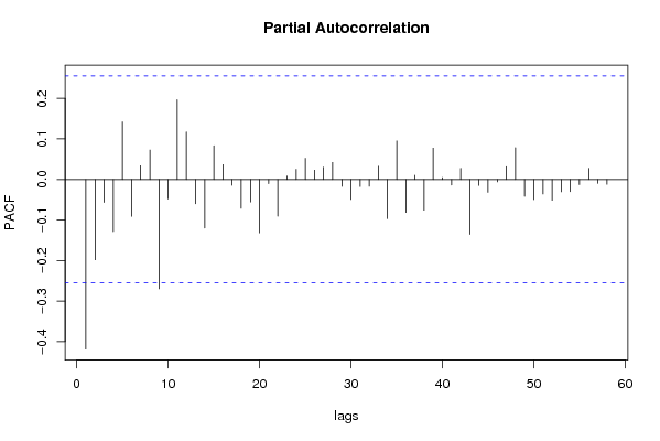
Title produced by software

(Partial) Autocorrelation Function

Date of computation

Fri, 19 Dec 2008 10:15:28 -0700

Cite this page as follows

Statistical Computations at FreeStatistics.org, Office for Research Development and Education, URL https://freestatistics.org/blog/index.php?v=date/2008/Dec/19/t12297069671eqlmgisn3gpo57.htm/, Retrieved Wed, 15 May 2024 13:50:08 +0000

Statistical Computations at FreeStatistics.org, Office for Research Development and Education, URL https://freestatistics.org/blog/index.php?pk=35226, Retrieved Wed, 15 May 2024 13:50:08 +0000

QR Codes:

Paste this QR Code to cite your computation.

Original text written by user:

IsPrivate?

No (this computation is public)

User-defined keywords

Estimated Impact

232

Family? (F = Feedback message, R = changed R code, M = changed R Module, P = changed Parameters, D = changed Data)

-     [Univariate Data Series] [data set] [2008-12-01 19:54:57] [b98453cac15ba1066b407e146608df68]
F RMP   [(Partial) Autocorrelation Function] [Taak 10 Stap 4] [2008-12-03 16:24:10] [6fea0e9a9b3b29a63badf2c274e82506]
-   P     [(Partial) Autocorrelation Function] [Identification an...] [2008-12-08 19:12:52] [79c17183721a40a589db5f9f561947d8]
- RMPD      [ARIMA Backward Selection] [arima backward el...] [2008-12-19 16:45:52] [44a98561a4b3e6ab8cd5a857b48b0914]
- RMPD          [(Partial) Autocorrelation Function] [(P)ACF olie] [2008-12-19 17:15:28] [1aceffc2fa350402d9e8f8edd757a2e8] [Current]
-   P             [(Partial) Autocorrelation Function] [pacf-acf olie] [2008-12-22 10:01:15] [44a98561a4b3e6ab8cd5a857b48b0914] 

Feedback Forum

Post a new message

Dataseries X:

Download CSV

Histogram

Boxplots

Summary of computational transaction
Raw Input	view raw input (R code)
Raw Output	view raw output of R engine
Computing time	1 seconds
R Server	'George Udny Yule' @ 72.249.76.132

\begin{tabular}{lllllllll}
\hline
Summary of computational transaction \tabularnewline
Raw Input & view raw input (R code)  \tabularnewline
Raw Output & view raw output of R engine  \tabularnewline
Computing time & 1 seconds \tabularnewline
R Server & 'George Udny Yule' @ 72.249.76.132 \tabularnewline
\hline
\end{tabular}
%Source: https://freestatistics.org/blog/index.php?pk=35226&T=0

[TABLE]
[ROW][C]Summary of computational transaction[/C][/ROW]
[ROW][C]Raw Input[/C][C]view raw input (R code) [/C][/ROW]
[ROW][C]Raw Output[/C][C]view raw output of R engine [/C][/ROW]
[ROW][C]Computing time[/C][C]1 seconds[/C][/ROW]
[ROW][C]R Server[/C][C]'George Udny Yule' @ 72.249.76.132[/C][/ROW]
[/TABLE]
Source: https://freestatistics.org/blog/index.php?pk=35226&T=0

Globally Unique Identifier (entire table): ba.freestatistics.org/blog/index.php?pk=35226&T=0

As an alternative you can also use a QR Code:

The GUIDs for individual cells are displayed in the table below:

Summary of computational transaction
Raw Input	view raw input (R code)
Raw Output	view raw output of R engine
Computing time	1 seconds
R Server	'George Udny Yule' @ 72.249.76.132

Autocorrelation Function
Time lag k	ACF(k)	T-STAT	P-value
1	-0.418581	-3.2152	0.001058
2	0.011595	0.0891	0.464666
3	0.032447	0.2492	0.402026
4	-0.097307	-0.7474	0.228888
5	0.205065	1.5751	0.060286
6	-0.211843	-1.6272	0.054512
7	0.125081	0.9608	0.170295
8	0.022994	0.1766	0.430207
9	-0.278992	-2.143	0.018125
10	0.225539	1.7324	0.044214
11	0.059364	0.456	0.325039
12	-0.008197	-0.063	0.475003
13	-0.088804	-0.6821	0.248917
14	-0.097196	-0.7466	0.229141
15	0.239564	1.8401	0.03539
16	-0.121482	-0.9331	0.177281
17	-0.005263	-0.0404	0.483944
18	0.023858	0.1833	0.427614
19	-0.088313	-0.6783	0.250104
20	-0.043164	-0.3315	0.370702
21	0.053878	0.4138	0.340243
22	0.016408	0.126	0.450067
23	0.039602	0.3042	0.381027
24	-0.137505	-1.0562	0.147592
25	0.096772	0.7433	0.230119
26	0.059599	0.4578	0.324394
27	-0.032224	-0.2475	0.402684
28	0.026325	0.2022	0.420224
29	-0.067166	-0.5159	0.303922
30	0.005247	0.0403	0.483993
31	-0.006738	-0.0518	0.47945
32	-0.007651	-0.0588	0.476666
33	0.086587	0.6651	0.254293
34	-0.148996	-1.1445	0.128527
35	0.111275	0.8547	0.198081
36	-0.084511	-0.6491	0.259382
37	0.079543	0.611	0.271779
38	-0.014778	-0.1135	0.455006
39	0.008787	0.0675	0.473209
40	0.014125	0.1085	0.456984
41	-0.070663	-0.5428	0.294665
42	0.084708	0.6507	0.258898
43	-0.105384	-0.8095	0.210749
44	0.042238	0.3244	0.373377
45	-0.037545	-0.2884	0.387031
46	-0.007918	-0.0608	0.475855
47	0.063455	0.4874	0.313888
48	-0.02293	-0.1761	0.430397
49	-0.011881	-0.0913	0.463797
50	0.036485	0.2802	0.390134
51	-0.071553	-0.5496	0.292331
52	0.06262	0.481	0.316151
53	-0.061864	-0.4752	0.318204
54	0.035538	0.273	0.392915
55	-0.035398	-0.2719	0.393326
56	0.015519	0.1192	0.452759
57	-0.000373	-0.0029	0.498861
58	2e-06	0	0.499993
59	NA	NA	NA
60	NA	NA	NA

\begin{tabular}{lllllllll}
\hline
Autocorrelation Function \tabularnewline
Time lag k & ACF(k) & T-STAT & P-value \tabularnewline
1 & -0.418581 & -3.2152 & 0.001058 \tabularnewline
2 & 0.011595 & 0.0891 & 0.464666 \tabularnewline
3 & 0.032447 & 0.2492 & 0.402026 \tabularnewline
4 & -0.097307 & -0.7474 & 0.228888 \tabularnewline
5 & 0.205065 & 1.5751 & 0.060286 \tabularnewline
6 & -0.211843 & -1.6272 & 0.054512 \tabularnewline
7 & 0.125081 & 0.9608 & 0.170295 \tabularnewline
8 & 0.022994 & 0.1766 & 0.430207 \tabularnewline
9 & -0.278992 & -2.143 & 0.018125 \tabularnewline
10 & 0.225539 & 1.7324 & 0.044214 \tabularnewline
11 & 0.059364 & 0.456 & 0.325039 \tabularnewline
12 & -0.008197 & -0.063 & 0.475003 \tabularnewline
13 & -0.088804 & -0.6821 & 0.248917 \tabularnewline
14 & -0.097196 & -0.7466 & 0.229141 \tabularnewline
15 & 0.239564 & 1.8401 & 0.03539 \tabularnewline
16 & -0.121482 & -0.9331 & 0.177281 \tabularnewline
17 & -0.005263 & -0.0404 & 0.483944 \tabularnewline
18 & 0.023858 & 0.1833 & 0.427614 \tabularnewline
19 & -0.088313 & -0.6783 & 0.250104 \tabularnewline
20 & -0.043164 & -0.3315 & 0.370702 \tabularnewline
21 & 0.053878 & 0.4138 & 0.340243 \tabularnewline
22 & 0.016408 & 0.126 & 0.450067 \tabularnewline
23 & 0.039602 & 0.3042 & 0.381027 \tabularnewline
24 & -0.137505 & -1.0562 & 0.147592 \tabularnewline
25 & 0.096772 & 0.7433 & 0.230119 \tabularnewline
26 & 0.059599 & 0.4578 & 0.324394 \tabularnewline
27 & -0.032224 & -0.2475 & 0.402684 \tabularnewline
28 & 0.026325 & 0.2022 & 0.420224 \tabularnewline
29 & -0.067166 & -0.5159 & 0.303922 \tabularnewline
30 & 0.005247 & 0.0403 & 0.483993 \tabularnewline
31 & -0.006738 & -0.0518 & 0.47945 \tabularnewline
32 & -0.007651 & -0.0588 & 0.476666 \tabularnewline
33 & 0.086587 & 0.6651 & 0.254293 \tabularnewline
34 & -0.148996 & -1.1445 & 0.128527 \tabularnewline
35 & 0.111275 & 0.8547 & 0.198081 \tabularnewline
36 & -0.084511 & -0.6491 & 0.259382 \tabularnewline
37 & 0.079543 & 0.611 & 0.271779 \tabularnewline
38 & -0.014778 & -0.1135 & 0.455006 \tabularnewline
39 & 0.008787 & 0.0675 & 0.473209 \tabularnewline
40 & 0.014125 & 0.1085 & 0.456984 \tabularnewline
41 & -0.070663 & -0.5428 & 0.294665 \tabularnewline
42 & 0.084708 & 0.6507 & 0.258898 \tabularnewline
43 & -0.105384 & -0.8095 & 0.210749 \tabularnewline
44 & 0.042238 & 0.3244 & 0.373377 \tabularnewline
45 & -0.037545 & -0.2884 & 0.387031 \tabularnewline
46 & -0.007918 & -0.0608 & 0.475855 \tabularnewline
47 & 0.063455 & 0.4874 & 0.313888 \tabularnewline
48 & -0.02293 & -0.1761 & 0.430397 \tabularnewline
49 & -0.011881 & -0.0913 & 0.463797 \tabularnewline
50 & 0.036485 & 0.2802 & 0.390134 \tabularnewline
51 & -0.071553 & -0.5496 & 0.292331 \tabularnewline
52 & 0.06262 & 0.481 & 0.316151 \tabularnewline
53 & -0.061864 & -0.4752 & 0.318204 \tabularnewline
54 & 0.035538 & 0.273 & 0.392915 \tabularnewline
55 & -0.035398 & -0.2719 & 0.393326 \tabularnewline
56 & 0.015519 & 0.1192 & 0.452759 \tabularnewline
57 & -0.000373 & -0.0029 & 0.498861 \tabularnewline
58 & 2e-06 & 0 & 0.499993 \tabularnewline
59 & NA & NA & NA \tabularnewline
60 & NA & NA & NA \tabularnewline
\hline
\end{tabular}
%Source: https://freestatistics.org/blog/index.php?pk=35226&T=1

[TABLE]
[ROW][C]Autocorrelation Function[/C][/ROW]
[ROW][C]Time lag k[/C][C]ACF(k)[/C][C]T-STAT[/C][C]P-value[/C][/ROW]
[ROW][C]1[/C][C]-0.418581[/C][C]-3.2152[/C][C]0.001058[/C][/ROW]
[ROW][C]2[/C][C]0.011595[/C][C]0.0891[/C][C]0.464666[/C][/ROW]
[ROW][C]3[/C][C]0.032447[/C][C]0.2492[/C][C]0.402026[/C][/ROW]
[ROW][C]4[/C][C]-0.097307[/C][C]-0.7474[/C][C]0.228888[/C][/ROW]
[ROW][C]5[/C][C]0.205065[/C][C]1.5751[/C][C]0.060286[/C][/ROW]
[ROW][C]6[/C][C]-0.211843[/C][C]-1.6272[/C][C]0.054512[/C][/ROW]
[ROW][C]7[/C][C]0.125081[/C][C]0.9608[/C][C]0.170295[/C][/ROW]
[ROW][C]8[/C][C]0.022994[/C][C]0.1766[/C][C]0.430207[/C][/ROW]
[ROW][C]9[/C][C]-0.278992[/C][C]-2.143[/C][C]0.018125[/C][/ROW]
[ROW][C]10[/C][C]0.225539[/C][C]1.7324[/C][C]0.044214[/C][/ROW]
[ROW][C]11[/C][C]0.059364[/C][C]0.456[/C][C]0.325039[/C][/ROW]
[ROW][C]12[/C][C]-0.008197[/C][C]-0.063[/C][C]0.475003[/C][/ROW]
[ROW][C]13[/C][C]-0.088804[/C][C]-0.6821[/C][C]0.248917[/C][/ROW]
[ROW][C]14[/C][C]-0.097196[/C][C]-0.7466[/C][C]0.229141[/C][/ROW]
[ROW][C]15[/C][C]0.239564[/C][C]1.8401[/C][C]0.03539[/C][/ROW]
[ROW][C]16[/C][C]-0.121482[/C][C]-0.9331[/C][C]0.177281[/C][/ROW]
[ROW][C]17[/C][C]-0.005263[/C][C]-0.0404[/C][C]0.483944[/C][/ROW]
[ROW][C]18[/C][C]0.023858[/C][C]0.1833[/C][C]0.427614[/C][/ROW]
[ROW][C]19[/C][C]-0.088313[/C][C]-0.6783[/C][C]0.250104[/C][/ROW]
[ROW][C]20[/C][C]-0.043164[/C][C]-0.3315[/C][C]0.370702[/C][/ROW]
[ROW][C]21[/C][C]0.053878[/C][C]0.4138[/C][C]0.340243[/C][/ROW]
[ROW][C]22[/C][C]0.016408[/C][C]0.126[/C][C]0.450067[/C][/ROW]
[ROW][C]23[/C][C]0.039602[/C][C]0.3042[/C][C]0.381027[/C][/ROW]
[ROW][C]24[/C][C]-0.137505[/C][C]-1.0562[/C][C]0.147592[/C][/ROW]
[ROW][C]25[/C][C]0.096772[/C][C]0.7433[/C][C]0.230119[/C][/ROW]
[ROW][C]26[/C][C]0.059599[/C][C]0.4578[/C][C]0.324394[/C][/ROW]
[ROW][C]27[/C][C]-0.032224[/C][C]-0.2475[/C][C]0.402684[/C][/ROW]
[ROW][C]28[/C][C]0.026325[/C][C]0.2022[/C][C]0.420224[/C][/ROW]
[ROW][C]29[/C][C]-0.067166[/C][C]-0.5159[/C][C]0.303922[/C][/ROW]
[ROW][C]30[/C][C]0.005247[/C][C]0.0403[/C][C]0.483993[/C][/ROW]
[ROW][C]31[/C][C]-0.006738[/C][C]-0.0518[/C][C]0.47945[/C][/ROW]
[ROW][C]32[/C][C]-0.007651[/C][C]-0.0588[/C][C]0.476666[/C][/ROW]
[ROW][C]33[/C][C]0.086587[/C][C]0.6651[/C][C]0.254293[/C][/ROW]
[ROW][C]34[/C][C]-0.148996[/C][C]-1.1445[/C][C]0.128527[/C][/ROW]
[ROW][C]35[/C][C]0.111275[/C][C]0.8547[/C][C]0.198081[/C][/ROW]
[ROW][C]36[/C][C]-0.084511[/C][C]-0.6491[/C][C]0.259382[/C][/ROW]
[ROW][C]37[/C][C]0.079543[/C][C]0.611[/C][C]0.271779[/C][/ROW]
[ROW][C]38[/C][C]-0.014778[/C][C]-0.1135[/C][C]0.455006[/C][/ROW]
[ROW][C]39[/C][C]0.008787[/C][C]0.0675[/C][C]0.473209[/C][/ROW]
[ROW][C]40[/C][C]0.014125[/C][C]0.1085[/C][C]0.456984[/C][/ROW]
[ROW][C]41[/C][C]-0.070663[/C][C]-0.5428[/C][C]0.294665[/C][/ROW]
[ROW][C]42[/C][C]0.084708[/C][C]0.6507[/C][C]0.258898[/C][/ROW]
[ROW][C]43[/C][C]-0.105384[/C][C]-0.8095[/C][C]0.210749[/C][/ROW]
[ROW][C]44[/C][C]0.042238[/C][C]0.3244[/C][C]0.373377[/C][/ROW]
[ROW][C]45[/C][C]-0.037545[/C][C]-0.2884[/C][C]0.387031[/C][/ROW]
[ROW][C]46[/C][C]-0.007918[/C][C]-0.0608[/C][C]0.475855[/C][/ROW]
[ROW][C]47[/C][C]0.063455[/C][C]0.4874[/C][C]0.313888[/C][/ROW]
[ROW][C]48[/C][C]-0.02293[/C][C]-0.1761[/C][C]0.430397[/C][/ROW]
[ROW][C]49[/C][C]-0.011881[/C][C]-0.0913[/C][C]0.463797[/C][/ROW]
[ROW][C]50[/C][C]0.036485[/C][C]0.2802[/C][C]0.390134[/C][/ROW]
[ROW][C]51[/C][C]-0.071553[/C][C]-0.5496[/C][C]0.292331[/C][/ROW]
[ROW][C]52[/C][C]0.06262[/C][C]0.481[/C][C]0.316151[/C][/ROW]
[ROW][C]53[/C][C]-0.061864[/C][C]-0.4752[/C][C]0.318204[/C][/ROW]
[ROW][C]54[/C][C]0.035538[/C][C]0.273[/C][C]0.392915[/C][/ROW]
[ROW][C]55[/C][C]-0.035398[/C][C]-0.2719[/C][C]0.393326[/C][/ROW]
[ROW][C]56[/C][C]0.015519[/C][C]0.1192[/C][C]0.452759[/C][/ROW]
[ROW][C]57[/C][C]-0.000373[/C][C]-0.0029[/C][C]0.498861[/C][/ROW]
[ROW][C]58[/C][C]2e-06[/C][C]0[/C][C]0.499993[/C][/ROW]
[ROW][C]59[/C][C]NA[/C][C]NA[/C][C]NA[/C][/ROW]
[ROW][C]60[/C][C]NA[/C][C]NA[/C][C]NA[/C][/ROW]
[/TABLE]
Source: https://freestatistics.org/blog/index.php?pk=35226&T=1

Globally Unique Identifier (entire table): ba.freestatistics.org/blog/index.php?pk=35226&T=1

As an alternative you can also use a QR Code:

The GUIDs for individual cells are displayed in the table below:

Autocorrelation Function
Time lag k	ACF(k)	T-STAT	P-value
1	-0.418581	-3.2152	0.001058
2	0.011595	0.0891	0.464666
3	0.032447	0.2492	0.402026
4	-0.097307	-0.7474	0.228888
5	0.205065	1.5751	0.060286
6	-0.211843	-1.6272	0.054512
7	0.125081	0.9608	0.170295
8	0.022994	0.1766	0.430207
9	-0.278992	-2.143	0.018125
10	0.225539	1.7324	0.044214
11	0.059364	0.456	0.325039
12	-0.008197	-0.063	0.475003
13	-0.088804	-0.6821	0.248917
14	-0.097196	-0.7466	0.229141
15	0.239564	1.8401	0.03539
16	-0.121482	-0.9331	0.177281
17	-0.005263	-0.0404	0.483944
18	0.023858	0.1833	0.427614
19	-0.088313	-0.6783	0.250104
20	-0.043164	-0.3315	0.370702
21	0.053878	0.4138	0.340243
22	0.016408	0.126	0.450067
23	0.039602	0.3042	0.381027
24	-0.137505	-1.0562	0.147592
25	0.096772	0.7433	0.230119
26	0.059599	0.4578	0.324394
27	-0.032224	-0.2475	0.402684
28	0.026325	0.2022	0.420224
29	-0.067166	-0.5159	0.303922
30	0.005247	0.0403	0.483993
31	-0.006738	-0.0518	0.47945
32	-0.007651	-0.0588	0.476666
33	0.086587	0.6651	0.254293
34	-0.148996	-1.1445	0.128527
35	0.111275	0.8547	0.198081
36	-0.084511	-0.6491	0.259382
37	0.079543	0.611	0.271779
38	-0.014778	-0.1135	0.455006
39	0.008787	0.0675	0.473209
40	0.014125	0.1085	0.456984
41	-0.070663	-0.5428	0.294665
42	0.084708	0.6507	0.258898
43	-0.105384	-0.8095	0.210749
44	0.042238	0.3244	0.373377
45	-0.037545	-0.2884	0.387031
46	-0.007918	-0.0608	0.475855
47	0.063455	0.4874	0.313888
48	-0.02293	-0.1761	0.430397
49	-0.011881	-0.0913	0.463797
50	0.036485	0.2802	0.390134
51	-0.071553	-0.5496	0.292331
52	0.06262	0.481	0.316151
53	-0.061864	-0.4752	0.318204
54	0.035538	0.273	0.392915
55	-0.035398	-0.2719	0.393326
56	0.015519	0.1192	0.452759
57	-0.000373	-0.0029	0.498861
58	2e-06	0	0.499993
59	NA	NA	NA
60	NA	NA	NA

Partial Autocorrelation Function
Time lag k	PACF(k)	T-STAT	P-value
1	-0.418581	-3.2152	0.001058
2	-0.198371	-1.5237	0.066461
3	-0.056506	-0.434	0.332925
4	-0.128754	-0.989	0.163356
5	0.141991	1.0907	0.13993
6	-0.091029	-0.6992	0.243585
7	0.033869	0.2602	0.397826
8	0.07261	0.5577	0.289571
9	-0.269827	-2.0726	0.021295
10	-0.048033	-0.369	0.356743
11	0.19666	1.5106	0.068117
12	0.117211	0.9003	0.185806
13	-0.059846	-0.4597	0.323717
14	-0.119814	-0.9203	0.18058
15	0.083143	0.6386	0.262767
16	0.036503	0.2804	0.390082
17	-0.014405	-0.1106	0.456136
18	-0.07115	-0.5465	0.293388
19	-0.055584	-0.4269	0.335487
20	-0.131584	-1.0107	0.15814
21	-0.010344	-0.0795	0.46847
22	-0.090494	-0.6951	0.244861
23	0.008354	0.0642	0.474527
24	0.025011	0.1921	0.424158
25	0.052125	0.4004	0.345161
26	0.023053	0.1771	0.430028
27	0.030107	0.2313	0.408958
28	0.041977	0.3224	0.374132
29	-0.017107	-0.1314	0.447954
30	-0.04954	-0.3805	0.352461
31	-0.017403	-0.1337	0.447058
32	-0.01681	-0.1291	0.448852
33	0.032636	0.2507	0.401465
34	-0.09669	-0.7427	0.230308
35	0.095164	0.731	0.233845
36	-0.081456	-0.6257	0.26697
37	0.010485	0.0805	0.46804
38	-0.076054	-0.5842	0.280664
39	0.077292	0.5937	0.277495
40	0.004718	0.0362	0.485608
41	-0.013857	-0.1064	0.457798
42	0.02744	0.2108	0.416897
43	-0.135583	-1.0414	0.150962
44	-0.014844	-0.114	0.454806
45	-0.031694	-0.2434	0.404251
46	-0.005901	-0.0453	0.482
47	0.031369	0.241	0.405215
48	0.07837	0.602	0.274749
49	-0.041668	-0.3201	0.375029
50	-0.049874	-0.3831	0.351514
51	-0.035846	-0.2753	0.392008
52	-0.051507	-0.3956	0.3469
53	-0.03055	-0.2347	0.407643
54	-0.029953	-0.2301	0.409415
55	-0.012842	-0.0986	0.46088
56	0.027448	0.2108	0.416873
57	-0.009666	-0.0742	0.470533
58	-0.012074	-0.0927	0.463212
59	NA	NA	NA
60	NA	NA	NA

\begin{tabular}{lllllllll}
\hline
Partial Autocorrelation Function \tabularnewline
Time lag k & PACF(k) & T-STAT & P-value \tabularnewline
1 & -0.418581 & -3.2152 & 0.001058 \tabularnewline
2 & -0.198371 & -1.5237 & 0.066461 \tabularnewline
3 & -0.056506 & -0.434 & 0.332925 \tabularnewline
4 & -0.128754 & -0.989 & 0.163356 \tabularnewline
5 & 0.141991 & 1.0907 & 0.13993 \tabularnewline
6 & -0.091029 & -0.6992 & 0.243585 \tabularnewline
7 & 0.033869 & 0.2602 & 0.397826 \tabularnewline
8 & 0.07261 & 0.5577 & 0.289571 \tabularnewline
9 & -0.269827 & -2.0726 & 0.021295 \tabularnewline
10 & -0.048033 & -0.369 & 0.356743 \tabularnewline
11 & 0.19666 & 1.5106 & 0.068117 \tabularnewline
12 & 0.117211 & 0.9003 & 0.185806 \tabularnewline
13 & -0.059846 & -0.4597 & 0.323717 \tabularnewline
14 & -0.119814 & -0.9203 & 0.18058 \tabularnewline
15 & 0.083143 & 0.6386 & 0.262767 \tabularnewline
16 & 0.036503 & 0.2804 & 0.390082 \tabularnewline
17 & -0.014405 & -0.1106 & 0.456136 \tabularnewline
18 & -0.07115 & -0.5465 & 0.293388 \tabularnewline
19 & -0.055584 & -0.4269 & 0.335487 \tabularnewline
20 & -0.131584 & -1.0107 & 0.15814 \tabularnewline
21 & -0.010344 & -0.0795 & 0.46847 \tabularnewline
22 & -0.090494 & -0.6951 & 0.244861 \tabularnewline
23 & 0.008354 & 0.0642 & 0.474527 \tabularnewline
24 & 0.025011 & 0.1921 & 0.424158 \tabularnewline
25 & 0.052125 & 0.4004 & 0.345161 \tabularnewline
26 & 0.023053 & 0.1771 & 0.430028 \tabularnewline
27 & 0.030107 & 0.2313 & 0.408958 \tabularnewline
28 & 0.041977 & 0.3224 & 0.374132 \tabularnewline
29 & -0.017107 & -0.1314 & 0.447954 \tabularnewline
30 & -0.04954 & -0.3805 & 0.352461 \tabularnewline
31 & -0.017403 & -0.1337 & 0.447058 \tabularnewline
32 & -0.01681 & -0.1291 & 0.448852 \tabularnewline
33 & 0.032636 & 0.2507 & 0.401465 \tabularnewline
34 & -0.09669 & -0.7427 & 0.230308 \tabularnewline
35 & 0.095164 & 0.731 & 0.233845 \tabularnewline
36 & -0.081456 & -0.6257 & 0.26697 \tabularnewline
37 & 0.010485 & 0.0805 & 0.46804 \tabularnewline
38 & -0.076054 & -0.5842 & 0.280664 \tabularnewline
39 & 0.077292 & 0.5937 & 0.277495 \tabularnewline
40 & 0.004718 & 0.0362 & 0.485608 \tabularnewline
41 & -0.013857 & -0.1064 & 0.457798 \tabularnewline
42 & 0.02744 & 0.2108 & 0.416897 \tabularnewline
43 & -0.135583 & -1.0414 & 0.150962 \tabularnewline
44 & -0.014844 & -0.114 & 0.454806 \tabularnewline
45 & -0.031694 & -0.2434 & 0.404251 \tabularnewline
46 & -0.005901 & -0.0453 & 0.482 \tabularnewline
47 & 0.031369 & 0.241 & 0.405215 \tabularnewline
48 & 0.07837 & 0.602 & 0.274749 \tabularnewline
49 & -0.041668 & -0.3201 & 0.375029 \tabularnewline
50 & -0.049874 & -0.3831 & 0.351514 \tabularnewline
51 & -0.035846 & -0.2753 & 0.392008 \tabularnewline
52 & -0.051507 & -0.3956 & 0.3469 \tabularnewline
53 & -0.03055 & -0.2347 & 0.407643 \tabularnewline
54 & -0.029953 & -0.2301 & 0.409415 \tabularnewline
55 & -0.012842 & -0.0986 & 0.46088 \tabularnewline
56 & 0.027448 & 0.2108 & 0.416873 \tabularnewline
57 & -0.009666 & -0.0742 & 0.470533 \tabularnewline
58 & -0.012074 & -0.0927 & 0.463212 \tabularnewline
59 & NA & NA & NA \tabularnewline
60 & NA & NA & NA \tabularnewline
\hline
\end{tabular}
%Source: https://freestatistics.org/blog/index.php?pk=35226&T=2

[TABLE]
[ROW][C]Partial Autocorrelation Function[/C][/ROW]
[ROW][C]Time lag k[/C][C]PACF(k)[/C][C]T-STAT[/C][C]P-value[/C][/ROW]
[ROW][C]1[/C][C]-0.418581[/C][C]-3.2152[/C][C]0.001058[/C][/ROW]
[ROW][C]2[/C][C]-0.198371[/C][C]-1.5237[/C][C]0.066461[/C][/ROW]
[ROW][C]3[/C][C]-0.056506[/C][C]-0.434[/C][C]0.332925[/C][/ROW]
[ROW][C]4[/C][C]-0.128754[/C][C]-0.989[/C][C]0.163356[/C][/ROW]
[ROW][C]5[/C][C]0.141991[/C][C]1.0907[/C][C]0.13993[/C][/ROW]
[ROW][C]6[/C][C]-0.091029[/C][C]-0.6992[/C][C]0.243585[/C][/ROW]
[ROW][C]7[/C][C]0.033869[/C][C]0.2602[/C][C]0.397826[/C][/ROW]
[ROW][C]8[/C][C]0.07261[/C][C]0.5577[/C][C]0.289571[/C][/ROW]
[ROW][C]9[/C][C]-0.269827[/C][C]-2.0726[/C][C]0.021295[/C][/ROW]
[ROW][C]10[/C][C]-0.048033[/C][C]-0.369[/C][C]0.356743[/C][/ROW]
[ROW][C]11[/C][C]0.19666[/C][C]1.5106[/C][C]0.068117[/C][/ROW]
[ROW][C]12[/C][C]0.117211[/C][C]0.9003[/C][C]0.185806[/C][/ROW]
[ROW][C]13[/C][C]-0.059846[/C][C]-0.4597[/C][C]0.323717[/C][/ROW]
[ROW][C]14[/C][C]-0.119814[/C][C]-0.9203[/C][C]0.18058[/C][/ROW]
[ROW][C]15[/C][C]0.083143[/C][C]0.6386[/C][C]0.262767[/C][/ROW]
[ROW][C]16[/C][C]0.036503[/C][C]0.2804[/C][C]0.390082[/C][/ROW]
[ROW][C]17[/C][C]-0.014405[/C][C]-0.1106[/C][C]0.456136[/C][/ROW]
[ROW][C]18[/C][C]-0.07115[/C][C]-0.5465[/C][C]0.293388[/C][/ROW]
[ROW][C]19[/C][C]-0.055584[/C][C]-0.4269[/C][C]0.335487[/C][/ROW]
[ROW][C]20[/C][C]-0.131584[/C][C]-1.0107[/C][C]0.15814[/C][/ROW]
[ROW][C]21[/C][C]-0.010344[/C][C]-0.0795[/C][C]0.46847[/C][/ROW]
[ROW][C]22[/C][C]-0.090494[/C][C]-0.6951[/C][C]0.244861[/C][/ROW]
[ROW][C]23[/C][C]0.008354[/C][C]0.0642[/C][C]0.474527[/C][/ROW]
[ROW][C]24[/C][C]0.025011[/C][C]0.1921[/C][C]0.424158[/C][/ROW]
[ROW][C]25[/C][C]0.052125[/C][C]0.4004[/C][C]0.345161[/C][/ROW]
[ROW][C]26[/C][C]0.023053[/C][C]0.1771[/C][C]0.430028[/C][/ROW]
[ROW][C]27[/C][C]0.030107[/C][C]0.2313[/C][C]0.408958[/C][/ROW]
[ROW][C]28[/C][C]0.041977[/C][C]0.3224[/C][C]0.374132[/C][/ROW]
[ROW][C]29[/C][C]-0.017107[/C][C]-0.1314[/C][C]0.447954[/C][/ROW]
[ROW][C]30[/C][C]-0.04954[/C][C]-0.3805[/C][C]0.352461[/C][/ROW]
[ROW][C]31[/C][C]-0.017403[/C][C]-0.1337[/C][C]0.447058[/C][/ROW]
[ROW][C]32[/C][C]-0.01681[/C][C]-0.1291[/C][C]0.448852[/C][/ROW]
[ROW][C]33[/C][C]0.032636[/C][C]0.2507[/C][C]0.401465[/C][/ROW]
[ROW][C]34[/C][C]-0.09669[/C][C]-0.7427[/C][C]0.230308[/C][/ROW]
[ROW][C]35[/C][C]0.095164[/C][C]0.731[/C][C]0.233845[/C][/ROW]
[ROW][C]36[/C][C]-0.081456[/C][C]-0.6257[/C][C]0.26697[/C][/ROW]
[ROW][C]37[/C][C]0.010485[/C][C]0.0805[/C][C]0.46804[/C][/ROW]
[ROW][C]38[/C][C]-0.076054[/C][C]-0.5842[/C][C]0.280664[/C][/ROW]
[ROW][C]39[/C][C]0.077292[/C][C]0.5937[/C][C]0.277495[/C][/ROW]
[ROW][C]40[/C][C]0.004718[/C][C]0.0362[/C][C]0.485608[/C][/ROW]
[ROW][C]41[/C][C]-0.013857[/C][C]-0.1064[/C][C]0.457798[/C][/ROW]
[ROW][C]42[/C][C]0.02744[/C][C]0.2108[/C][C]0.416897[/C][/ROW]
[ROW][C]43[/C][C]-0.135583[/C][C]-1.0414[/C][C]0.150962[/C][/ROW]
[ROW][C]44[/C][C]-0.014844[/C][C]-0.114[/C][C]0.454806[/C][/ROW]
[ROW][C]45[/C][C]-0.031694[/C][C]-0.2434[/C][C]0.404251[/C][/ROW]
[ROW][C]46[/C][C]-0.005901[/C][C]-0.0453[/C][C]0.482[/C][/ROW]
[ROW][C]47[/C][C]0.031369[/C][C]0.241[/C][C]0.405215[/C][/ROW]
[ROW][C]48[/C][C]0.07837[/C][C]0.602[/C][C]0.274749[/C][/ROW]
[ROW][C]49[/C][C]-0.041668[/C][C]-0.3201[/C][C]0.375029[/C][/ROW]
[ROW][C]50[/C][C]-0.049874[/C][C]-0.3831[/C][C]0.351514[/C][/ROW]
[ROW][C]51[/C][C]-0.035846[/C][C]-0.2753[/C][C]0.392008[/C][/ROW]
[ROW][C]52[/C][C]-0.051507[/C][C]-0.3956[/C][C]0.3469[/C][/ROW]
[ROW][C]53[/C][C]-0.03055[/C][C]-0.2347[/C][C]0.407643[/C][/ROW]
[ROW][C]54[/C][C]-0.029953[/C][C]-0.2301[/C][C]0.409415[/C][/ROW]
[ROW][C]55[/C][C]-0.012842[/C][C]-0.0986[/C][C]0.46088[/C][/ROW]
[ROW][C]56[/C][C]0.027448[/C][C]0.2108[/C][C]0.416873[/C][/ROW]
[ROW][C]57[/C][C]-0.009666[/C][C]-0.0742[/C][C]0.470533[/C][/ROW]
[ROW][C]58[/C][C]-0.012074[/C][C]-0.0927[/C][C]0.463212[/C][/ROW]
[ROW][C]59[/C][C]NA[/C][C]NA[/C][C]NA[/C][/ROW]
[ROW][C]60[/C][C]NA[/C][C]NA[/C][C]NA[/C][/ROW]
[/TABLE]
Source: https://freestatistics.org/blog/index.php?pk=35226&T=2

Globally Unique Identifier (entire table): ba.freestatistics.org/blog/index.php?pk=35226&T=2

As an alternative you can also use a QR Code:

The GUIDs for individual cells are displayed in the table below:

Partial Autocorrelation Function
Time lag k	PACF(k)	T-STAT	P-value
1	-0.418581	-3.2152	0.001058
2	-0.198371	-1.5237	0.066461
3	-0.056506	-0.434	0.332925
4	-0.128754	-0.989	0.163356
5	0.141991	1.0907	0.13993
6	-0.091029	-0.6992	0.243585
7	0.033869	0.2602	0.397826
8	0.07261	0.5577	0.289571
9	-0.269827	-2.0726	0.021295
10	-0.048033	-0.369	0.356743
11	0.19666	1.5106	0.068117
12	0.117211	0.9003	0.185806
13	-0.059846	-0.4597	0.323717
14	-0.119814	-0.9203	0.18058
15	0.083143	0.6386	0.262767
16	0.036503	0.2804	0.390082
17	-0.014405	-0.1106	0.456136
18	-0.07115	-0.5465	0.293388
19	-0.055584	-0.4269	0.335487
20	-0.131584	-1.0107	0.15814
21	-0.010344	-0.0795	0.46847
22	-0.090494	-0.6951	0.244861
23	0.008354	0.0642	0.474527
24	0.025011	0.1921	0.424158
25	0.052125	0.4004	0.345161
26	0.023053	0.1771	0.430028
27	0.030107	0.2313	0.408958
28	0.041977	0.3224	0.374132
29	-0.017107	-0.1314	0.447954
30	-0.04954	-0.3805	0.352461
31	-0.017403	-0.1337	0.447058
32	-0.01681	-0.1291	0.448852
33	0.032636	0.2507	0.401465
34	-0.09669	-0.7427	0.230308
35	0.095164	0.731	0.233845
36	-0.081456	-0.6257	0.26697
37	0.010485	0.0805	0.46804
38	-0.076054	-0.5842	0.280664
39	0.077292	0.5937	0.277495
40	0.004718	0.0362	0.485608
41	-0.013857	-0.1064	0.457798
42	0.02744	0.2108	0.416897
43	-0.135583	-1.0414	0.150962
44	-0.014844	-0.114	0.454806
45	-0.031694	-0.2434	0.404251
46	-0.005901	-0.0453	0.482
47	0.031369	0.241	0.405215
48	0.07837	0.602	0.274749
49	-0.041668	-0.3201	0.375029
50	-0.049874	-0.3831	0.351514
51	-0.035846	-0.2753	0.392008
52	-0.051507	-0.3956	0.3469
53	-0.03055	-0.2347	0.407643
54	-0.029953	-0.2301	0.409415
55	-0.012842	-0.0986	0.46088
56	0.027448	0.2108	0.416873
57	-0.009666	-0.0742	0.470533
58	-0.012074	-0.0927	0.463212
59	NA	NA	NA
60	NA	NA	NA

Figure 1

PNG link

Postscript link

PDF link

Figure 2

PNG link

Postscript link

PDF link

Parameters (Session):

par1 = 60 ; par2 = -0.1 ; par3 = 2 ; par4 = 0 ; par5 = 12 ;

Parameters (R input):

par1 = 60 ; par2 = -0.1 ; par3 = 2 ; par4 = 0 ; par5 = 12 ;

R code (references can be found in the software module):

if (par1 == 'Default') {
par1 = 10*log10(length(x))
} else {
par1 <- as.numeric(par1)
}
par2 <- as.numeric(par2)
par3 <- as.numeric(par3)
par4 <- as.numeric(par4)
par5 <- as.numeric(par5)
if (par2 == 0) {
x <- log(x)
} else {
x <- (x ^ par2 - 1) / par2
}
if (par3 > 0) x <- diff(x,lag=1,difference=par3)
if (par4 > 0) x <- diff(x,lag=par5,difference=par4)
bitmap(file='pic1.png')
racf <- acf(x,par1,main='Autocorrelation',xlab='lags',ylab='ACF')
dev.off()
bitmap(file='pic2.png')
rpacf <- pacf(x,par1,main='Partial Autocorrelation',xlab='lags',ylab='PACF')
dev.off()
(myacf <- c(racf$acf))
(mypacf <- c(rpacf$acf))
lengthx <- length(x)
sqrtn <- sqrt(lengthx)
load(file='createtable')
a<-table.start()
a<-table.row.start(a)
a<-table.element(a,'Autocorrelation Function',4,TRUE)
a<-table.row.end(a)
a<-table.row.start(a)
a<-table.element(a,'Time lag k',header=TRUE)
a<-table.element(a,hyperlink('basics.htm','ACF(k)','click here for more information about the Autocorrelation Function'),header=TRUE)
a<-table.element(a,'T-STAT',header=TRUE)
a<-table.element(a,'P-value',header=TRUE)
a<-table.row.end(a)
for (i in 2:(par1+1)) {
a<-table.row.start(a)
a<-table.element(a,i-1,header=TRUE)
a<-table.element(a,round(myacf[i],6))
mytstat <- myacf[i]*sqrtn
a<-table.element(a,round(mytstat,4))
a<-table.element(a,round(1-pt(abs(mytstat),lengthx),6))
a<-table.row.end(a)
}
a<-table.end(a)
table.save(a,file='mytable.tab')
a<-table.start()
a<-table.row.start(a)
a<-table.element(a,'Partial Autocorrelation Function',4,TRUE)
a<-table.row.end(a)
a<-table.row.start(a)
a<-table.element(a,'Time lag k',header=TRUE)
a<-table.element(a,hyperlink('basics.htm','PACF(k)','click here for more information about the Partial Autocorrelation Function'),header=TRUE)
a<-table.element(a,'T-STAT',header=TRUE)
a<-table.element(a,'P-value',header=TRUE)
a<-table.row.end(a)
for (i in 1:par1) {
a<-table.row.start(a)
a<-table.element(a,i,header=TRUE)
a<-table.element(a,round(mypacf[i],6))
mytstat <- mypacf[i]*sqrtn
a<-table.element(a,round(mytstat,4))
a<-table.element(a,round(1-pt(abs(mytstat),lengthx),6))
a<-table.row.end(a)
}
a<-table.end(a)
table.save(a,file='mytable1.tab')

Free Statistics

Description of Statistical Computation

Tree of Dependent Computations

Dataset

Tables (Output of Computation)

Figures (Output of Computation)

Input Parameters & R Code