Repository of Reproducible Computations

Free Statistics

of Irreproducible Research!

Author's title

Author

*Unverified author*

R Software Module

rwasp_autocorrelation.wasp

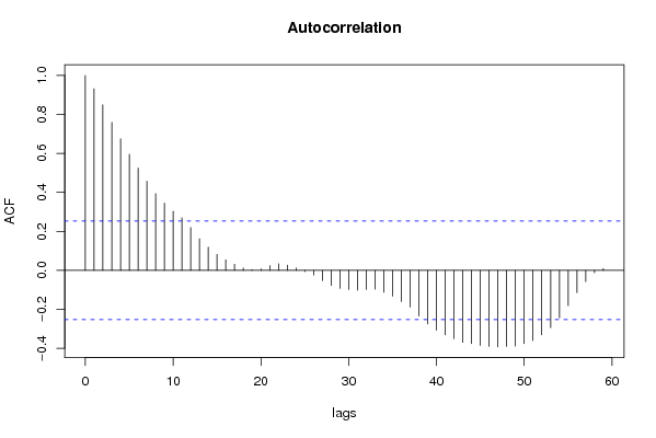
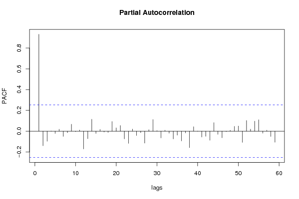
Title produced by software

(Partial) Autocorrelation Function

Date of computation

Fri, 19 Dec 2008 08:25:09 -0700

Cite this page as follows

Statistical Computations at FreeStatistics.org, Office for Research Development and Education, URL https://freestatistics.org/blog/index.php?v=date/2008/Dec/19/t1229700348aweh0kq0531bswa.htm/, Retrieved Wed, 15 May 2024 12:10:18 +0000

Statistical Computations at FreeStatistics.org, Office for Research Development and Education, URL https://freestatistics.org/blog/index.php?pk=35184, Retrieved Wed, 15 May 2024 12:10:18 +0000

QR Codes:

Paste this QR Code to cite your computation.

Original text written by user:

IsPrivate?

No (this computation is public)

User-defined keywords

Estimated Impact

233

Family? (F = Feedback message, R = changed R code, M = changed R Module, P = changed Parameters, D = changed Data)

-     [Univariate Data Series] [data set] [2008-12-01 19:54:57] [b98453cac15ba1066b407e146608df68]
- RMP   [Standard Deviation-Mean Plot] [Identification an...] [2008-12-07 12:51:02] [b943bd7078334192ff8343563ee31113]
- RM      [Variance Reduction Matrix] [Identification an...] [2008-12-07 12:57:34] [b943bd7078334192ff8343563ee31113]
- RMP       [(Partial) Autocorrelation Function] [Identification an...] [2008-12-07 13:03:39] [b943bd7078334192ff8343563ee31113]
-    D        [(Partial) Autocorrelation Function] [Correlation funct...] [2008-12-19 14:39:31] [74be16979710d4c4e7c6647856088456]
-   PD          [(Partial) Autocorrelation Function] [] [2008-12-19 14:46:38] [74be16979710d4c4e7c6647856088456]
-   P               [(Partial) Autocorrelation Function] [ACF d=0,D=0] [2008-12-19 15:25:09] [d41d8cd98f00b204e9800998ecf8427e] [Current]
-   P                 [(Partial) Autocorrelation Function] [ACF d=1,D=0] [2008-12-19 15:27:04] [74be16979710d4c4e7c6647856088456] 

Feedback Forum

Post a new message

Dataseries X:

Download CSV

Histogram

Boxplots

Summary of computational transaction
Raw Input	view raw input (R code)
Raw Output	view raw output of R engine
Computing time	1 seconds
R Server	'Gwilym Jenkins' @ 72.249.127.135

\begin{tabular}{lllllllll}
\hline
Summary of computational transaction \tabularnewline
Raw Input & view raw input (R code)  \tabularnewline
Raw Output & view raw output of R engine  \tabularnewline
Computing time & 1 seconds \tabularnewline
R Server & 'Gwilym Jenkins' @ 72.249.127.135 \tabularnewline
\hline
\end{tabular}
%Source: https://freestatistics.org/blog/index.php?pk=35184&T=0

[TABLE]
[ROW][C]Summary of computational transaction[/C][/ROW]
[ROW][C]Raw Input[/C][C]view raw input (R code) [/C][/ROW]
[ROW][C]Raw Output[/C][C]view raw output of R engine [/C][/ROW]
[ROW][C]Computing time[/C][C]1 seconds[/C][/ROW]
[ROW][C]R Server[/C][C]'Gwilym Jenkins' @ 72.249.127.135[/C][/ROW]
[/TABLE]
Source: https://freestatistics.org/blog/index.php?pk=35184&T=0

Globally Unique Identifier (entire table): ba.freestatistics.org/blog/index.php?pk=35184&T=0

As an alternative you can also use a QR Code:

The GUIDs for individual cells are displayed in the table below:

Summary of computational transaction
Raw Input	view raw input (R code)
Raw Output	view raw output of R engine
Computing time	1 seconds
R Server	'Gwilym Jenkins' @ 72.249.127.135

Autocorrelation Function
Time lag k	ACF(k)	T-STAT	P-value
1	0.931722	7.2171	0
2	0.849666	6.5815	0
3	0.759602	5.8839	0
4	0.675185	5.23	1e-06
5	0.595164	4.6101	1.1e-05
6	0.52541	4.0698	7e-05
7	0.45704	3.5402	0.00039
8	0.393725	3.0498	0.001703
9	0.344983	2.6722	0.004844
10	0.303475	2.3507	0.011021
11	0.26993	2.0909	0.020392
12	0.219553	1.7006	0.047093
13	0.16199	1.2548	0.107214
14	0.119387	0.9248	0.179396
15	0.081938	0.6347	0.264023
16	0.054095	0.419	0.33835
17	0.031659	0.2452	0.403558
18	0.01192	0.0923	0.46337
19	0.003901	0.0302	0.487998
20	0.00782	0.0606	0.475949
21	0.024203	0.1875	0.425959
22	0.033903	0.2626	0.396875
23	0.026511	0.2054	0.418995
24	0.011709	0.0907	0.464018
25	-0.006376	-0.0494	0.480388
26	-0.023749	-0.184	0.427334
27	-0.052731	-0.4085	0.342197
28	-0.077274	-0.5986	0.275858
29	-0.092111	-0.7135	0.239155
30	-0.098101	-0.7599	0.225149
31	-0.102315	-0.7925	0.215587
32	-0.098289	-0.7613	0.224717
33	-0.096706	-0.7491	0.228367
34	-0.112506	-0.8715	0.193486
35	-0.132474	-1.0261	0.154472
36	-0.160245	-1.2412	0.109672
37	-0.188266	-1.4583	0.074987
38	-0.234442	-1.816	0.037185
39	-0.274987	-2.13	0.018639
40	-0.307074	-2.3786	0.01029
41	-0.330788	-2.5623	0.006464
42	-0.350981	-2.7187	0.004279
43	-0.369391	-2.8613	0.0029
44	-0.376124	-2.9134	0.002508
45	-0.3848	-2.9806	0.002075
46	-0.390019	-3.0211	0.001849
47	-0.391964	-3.0361	0.001771
48	-0.390203	-3.0225	0.001842
49	-0.388353	-3.0082	0.001919
50	-0.376185	-2.9139	0.002504
51	-0.360712	-2.7941	0.003489
52	-0.33073	-2.5618	0.006471
53	-0.294097	-2.2781	0.013149
54	-0.244147	-1.8912	0.031717
55	-0.181746	-1.4078	0.082175
56	-0.114948	-0.8904	0.188409
57	-0.058048	-0.4496	0.327296
58	-0.012414	-0.0962	0.461858
59	0.008805	0.0682	0.472924
60	NA	NA	NA

\begin{tabular}{lllllllll}
\hline
Autocorrelation Function \tabularnewline
Time lag k & ACF(k) & T-STAT & P-value \tabularnewline
1 & 0.931722 & 7.2171 & 0 \tabularnewline
2 & 0.849666 & 6.5815 & 0 \tabularnewline
3 & 0.759602 & 5.8839 & 0 \tabularnewline
4 & 0.675185 & 5.23 & 1e-06 \tabularnewline
5 & 0.595164 & 4.6101 & 1.1e-05 \tabularnewline
6 & 0.52541 & 4.0698 & 7e-05 \tabularnewline
7 & 0.45704 & 3.5402 & 0.00039 \tabularnewline
8 & 0.393725 & 3.0498 & 0.001703 \tabularnewline
9 & 0.344983 & 2.6722 & 0.004844 \tabularnewline
10 & 0.303475 & 2.3507 & 0.011021 \tabularnewline
11 & 0.26993 & 2.0909 & 0.020392 \tabularnewline
12 & 0.219553 & 1.7006 & 0.047093 \tabularnewline
13 & 0.16199 & 1.2548 & 0.107214 \tabularnewline
14 & 0.119387 & 0.9248 & 0.179396 \tabularnewline
15 & 0.081938 & 0.6347 & 0.264023 \tabularnewline
16 & 0.054095 & 0.419 & 0.33835 \tabularnewline
17 & 0.031659 & 0.2452 & 0.403558 \tabularnewline
18 & 0.01192 & 0.0923 & 0.46337 \tabularnewline
19 & 0.003901 & 0.0302 & 0.487998 \tabularnewline
20 & 0.00782 & 0.0606 & 0.475949 \tabularnewline
21 & 0.024203 & 0.1875 & 0.425959 \tabularnewline
22 & 0.033903 & 0.2626 & 0.396875 \tabularnewline
23 & 0.026511 & 0.2054 & 0.418995 \tabularnewline
24 & 0.011709 & 0.0907 & 0.464018 \tabularnewline
25 & -0.006376 & -0.0494 & 0.480388 \tabularnewline
26 & -0.023749 & -0.184 & 0.427334 \tabularnewline
27 & -0.052731 & -0.4085 & 0.342197 \tabularnewline
28 & -0.077274 & -0.5986 & 0.275858 \tabularnewline
29 & -0.092111 & -0.7135 & 0.239155 \tabularnewline
30 & -0.098101 & -0.7599 & 0.225149 \tabularnewline
31 & -0.102315 & -0.7925 & 0.215587 \tabularnewline
32 & -0.098289 & -0.7613 & 0.224717 \tabularnewline
33 & -0.096706 & -0.7491 & 0.228367 \tabularnewline
34 & -0.112506 & -0.8715 & 0.193486 \tabularnewline
35 & -0.132474 & -1.0261 & 0.154472 \tabularnewline
36 & -0.160245 & -1.2412 & 0.109672 \tabularnewline
37 & -0.188266 & -1.4583 & 0.074987 \tabularnewline
38 & -0.234442 & -1.816 & 0.037185 \tabularnewline
39 & -0.274987 & -2.13 & 0.018639 \tabularnewline
40 & -0.307074 & -2.3786 & 0.01029 \tabularnewline
41 & -0.330788 & -2.5623 & 0.006464 \tabularnewline
42 & -0.350981 & -2.7187 & 0.004279 \tabularnewline
43 & -0.369391 & -2.8613 & 0.0029 \tabularnewline
44 & -0.376124 & -2.9134 & 0.002508 \tabularnewline
45 & -0.3848 & -2.9806 & 0.002075 \tabularnewline
46 & -0.390019 & -3.0211 & 0.001849 \tabularnewline
47 & -0.391964 & -3.0361 & 0.001771 \tabularnewline
48 & -0.390203 & -3.0225 & 0.001842 \tabularnewline
49 & -0.388353 & -3.0082 & 0.001919 \tabularnewline
50 & -0.376185 & -2.9139 & 0.002504 \tabularnewline
51 & -0.360712 & -2.7941 & 0.003489 \tabularnewline
52 & -0.33073 & -2.5618 & 0.006471 \tabularnewline
53 & -0.294097 & -2.2781 & 0.013149 \tabularnewline
54 & -0.244147 & -1.8912 & 0.031717 \tabularnewline
55 & -0.181746 & -1.4078 & 0.082175 \tabularnewline
56 & -0.114948 & -0.8904 & 0.188409 \tabularnewline
57 & -0.058048 & -0.4496 & 0.327296 \tabularnewline
58 & -0.012414 & -0.0962 & 0.461858 \tabularnewline
59 & 0.008805 & 0.0682 & 0.472924 \tabularnewline
60 & NA & NA & NA \tabularnewline
\hline
\end{tabular}
%Source: https://freestatistics.org/blog/index.php?pk=35184&T=1

[TABLE]
[ROW][C]Autocorrelation Function[/C][/ROW]
[ROW][C]Time lag k[/C][C]ACF(k)[/C][C]T-STAT[/C][C]P-value[/C][/ROW]
[ROW][C]1[/C][C]0.931722[/C][C]7.2171[/C][C]0[/C][/ROW]
[ROW][C]2[/C][C]0.849666[/C][C]6.5815[/C][C]0[/C][/ROW]
[ROW][C]3[/C][C]0.759602[/C][C]5.8839[/C][C]0[/C][/ROW]
[ROW][C]4[/C][C]0.675185[/C][C]5.23[/C][C]1e-06[/C][/ROW]
[ROW][C]5[/C][C]0.595164[/C][C]4.6101[/C][C]1.1e-05[/C][/ROW]
[ROW][C]6[/C][C]0.52541[/C][C]4.0698[/C][C]7e-05[/C][/ROW]
[ROW][C]7[/C][C]0.45704[/C][C]3.5402[/C][C]0.00039[/C][/ROW]
[ROW][C]8[/C][C]0.393725[/C][C]3.0498[/C][C]0.001703[/C][/ROW]
[ROW][C]9[/C][C]0.344983[/C][C]2.6722[/C][C]0.004844[/C][/ROW]
[ROW][C]10[/C][C]0.303475[/C][C]2.3507[/C][C]0.011021[/C][/ROW]
[ROW][C]11[/C][C]0.26993[/C][C]2.0909[/C][C]0.020392[/C][/ROW]
[ROW][C]12[/C][C]0.219553[/C][C]1.7006[/C][C]0.047093[/C][/ROW]
[ROW][C]13[/C][C]0.16199[/C][C]1.2548[/C][C]0.107214[/C][/ROW]
[ROW][C]14[/C][C]0.119387[/C][C]0.9248[/C][C]0.179396[/C][/ROW]
[ROW][C]15[/C][C]0.081938[/C][C]0.6347[/C][C]0.264023[/C][/ROW]
[ROW][C]16[/C][C]0.054095[/C][C]0.419[/C][C]0.33835[/C][/ROW]
[ROW][C]17[/C][C]0.031659[/C][C]0.2452[/C][C]0.403558[/C][/ROW]
[ROW][C]18[/C][C]0.01192[/C][C]0.0923[/C][C]0.46337[/C][/ROW]
[ROW][C]19[/C][C]0.003901[/C][C]0.0302[/C][C]0.487998[/C][/ROW]
[ROW][C]20[/C][C]0.00782[/C][C]0.0606[/C][C]0.475949[/C][/ROW]
[ROW][C]21[/C][C]0.024203[/C][C]0.1875[/C][C]0.425959[/C][/ROW]
[ROW][C]22[/C][C]0.033903[/C][C]0.2626[/C][C]0.396875[/C][/ROW]
[ROW][C]23[/C][C]0.026511[/C][C]0.2054[/C][C]0.418995[/C][/ROW]
[ROW][C]24[/C][C]0.011709[/C][C]0.0907[/C][C]0.464018[/C][/ROW]
[ROW][C]25[/C][C]-0.006376[/C][C]-0.0494[/C][C]0.480388[/C][/ROW]
[ROW][C]26[/C][C]-0.023749[/C][C]-0.184[/C][C]0.427334[/C][/ROW]
[ROW][C]27[/C][C]-0.052731[/C][C]-0.4085[/C][C]0.342197[/C][/ROW]
[ROW][C]28[/C][C]-0.077274[/C][C]-0.5986[/C][C]0.275858[/C][/ROW]
[ROW][C]29[/C][C]-0.092111[/C][C]-0.7135[/C][C]0.239155[/C][/ROW]
[ROW][C]30[/C][C]-0.098101[/C][C]-0.7599[/C][C]0.225149[/C][/ROW]
[ROW][C]31[/C][C]-0.102315[/C][C]-0.7925[/C][C]0.215587[/C][/ROW]
[ROW][C]32[/C][C]-0.098289[/C][C]-0.7613[/C][C]0.224717[/C][/ROW]
[ROW][C]33[/C][C]-0.096706[/C][C]-0.7491[/C][C]0.228367[/C][/ROW]
[ROW][C]34[/C][C]-0.112506[/C][C]-0.8715[/C][C]0.193486[/C][/ROW]
[ROW][C]35[/C][C]-0.132474[/C][C]-1.0261[/C][C]0.154472[/C][/ROW]
[ROW][C]36[/C][C]-0.160245[/C][C]-1.2412[/C][C]0.109672[/C][/ROW]
[ROW][C]37[/C][C]-0.188266[/C][C]-1.4583[/C][C]0.074987[/C][/ROW]
[ROW][C]38[/C][C]-0.234442[/C][C]-1.816[/C][C]0.037185[/C][/ROW]
[ROW][C]39[/C][C]-0.274987[/C][C]-2.13[/C][C]0.018639[/C][/ROW]
[ROW][C]40[/C][C]-0.307074[/C][C]-2.3786[/C][C]0.01029[/C][/ROW]
[ROW][C]41[/C][C]-0.330788[/C][C]-2.5623[/C][C]0.006464[/C][/ROW]
[ROW][C]42[/C][C]-0.350981[/C][C]-2.7187[/C][C]0.004279[/C][/ROW]
[ROW][C]43[/C][C]-0.369391[/C][C]-2.8613[/C][C]0.0029[/C][/ROW]
[ROW][C]44[/C][C]-0.376124[/C][C]-2.9134[/C][C]0.002508[/C][/ROW]
[ROW][C]45[/C][C]-0.3848[/C][C]-2.9806[/C][C]0.002075[/C][/ROW]
[ROW][C]46[/C][C]-0.390019[/C][C]-3.0211[/C][C]0.001849[/C][/ROW]
[ROW][C]47[/C][C]-0.391964[/C][C]-3.0361[/C][C]0.001771[/C][/ROW]
[ROW][C]48[/C][C]-0.390203[/C][C]-3.0225[/C][C]0.001842[/C][/ROW]
[ROW][C]49[/C][C]-0.388353[/C][C]-3.0082[/C][C]0.001919[/C][/ROW]
[ROW][C]50[/C][C]-0.376185[/C][C]-2.9139[/C][C]0.002504[/C][/ROW]
[ROW][C]51[/C][C]-0.360712[/C][C]-2.7941[/C][C]0.003489[/C][/ROW]
[ROW][C]52[/C][C]-0.33073[/C][C]-2.5618[/C][C]0.006471[/C][/ROW]
[ROW][C]53[/C][C]-0.294097[/C][C]-2.2781[/C][C]0.013149[/C][/ROW]
[ROW][C]54[/C][C]-0.244147[/C][C]-1.8912[/C][C]0.031717[/C][/ROW]
[ROW][C]55[/C][C]-0.181746[/C][C]-1.4078[/C][C]0.082175[/C][/ROW]
[ROW][C]56[/C][C]-0.114948[/C][C]-0.8904[/C][C]0.188409[/C][/ROW]
[ROW][C]57[/C][C]-0.058048[/C][C]-0.4496[/C][C]0.327296[/C][/ROW]
[ROW][C]58[/C][C]-0.012414[/C][C]-0.0962[/C][C]0.461858[/C][/ROW]
[ROW][C]59[/C][C]0.008805[/C][C]0.0682[/C][C]0.472924[/C][/ROW]
[ROW][C]60[/C][C]NA[/C][C]NA[/C][C]NA[/C][/ROW]
[/TABLE]
Source: https://freestatistics.org/blog/index.php?pk=35184&T=1

Globally Unique Identifier (entire table): ba.freestatistics.org/blog/index.php?pk=35184&T=1

As an alternative you can also use a QR Code:

The GUIDs for individual cells are displayed in the table below:

Autocorrelation Function
Time lag k	ACF(k)	T-STAT	P-value
1	0.931722	7.2171	0
2	0.849666	6.5815	0
3	0.759602	5.8839	0
4	0.675185	5.23	1e-06
5	0.595164	4.6101	1.1e-05
6	0.52541	4.0698	7e-05
7	0.45704	3.5402	0.00039
8	0.393725	3.0498	0.001703
9	0.344983	2.6722	0.004844
10	0.303475	2.3507	0.011021
11	0.26993	2.0909	0.020392
12	0.219553	1.7006	0.047093
13	0.16199	1.2548	0.107214
14	0.119387	0.9248	0.179396
15	0.081938	0.6347	0.264023
16	0.054095	0.419	0.33835
17	0.031659	0.2452	0.403558
18	0.01192	0.0923	0.46337
19	0.003901	0.0302	0.487998
20	0.00782	0.0606	0.475949
21	0.024203	0.1875	0.425959
22	0.033903	0.2626	0.396875
23	0.026511	0.2054	0.418995
24	0.011709	0.0907	0.464018
25	-0.006376	-0.0494	0.480388
26	-0.023749	-0.184	0.427334
27	-0.052731	-0.4085	0.342197
28	-0.077274	-0.5986	0.275858
29	-0.092111	-0.7135	0.239155
30	-0.098101	-0.7599	0.225149
31	-0.102315	-0.7925	0.215587
32	-0.098289	-0.7613	0.224717
33	-0.096706	-0.7491	0.228367
34	-0.112506	-0.8715	0.193486
35	-0.132474	-1.0261	0.154472
36	-0.160245	-1.2412	0.109672
37	-0.188266	-1.4583	0.074987
38	-0.234442	-1.816	0.037185
39	-0.274987	-2.13	0.018639
40	-0.307074	-2.3786	0.01029
41	-0.330788	-2.5623	0.006464
42	-0.350981	-2.7187	0.004279
43	-0.369391	-2.8613	0.0029
44	-0.376124	-2.9134	0.002508
45	-0.3848	-2.9806	0.002075
46	-0.390019	-3.0211	0.001849
47	-0.391964	-3.0361	0.001771
48	-0.390203	-3.0225	0.001842
49	-0.388353	-3.0082	0.001919
50	-0.376185	-2.9139	0.002504
51	-0.360712	-2.7941	0.003489
52	-0.33073	-2.5618	0.006471
53	-0.294097	-2.2781	0.013149
54	-0.244147	-1.8912	0.031717
55	-0.181746	-1.4078	0.082175
56	-0.114948	-0.8904	0.188409
57	-0.058048	-0.4496	0.327296
58	-0.012414	-0.0962	0.461858
59	0.008805	0.0682	0.472924
60	NA	NA	NA

Partial Autocorrelation Function
Time lag k	PACF(k)	T-STAT	P-value
1	0.931722	7.2171	0
2	-0.139806	-1.0829	0.141586
3	-0.096415	-0.7468	0.229043
4	0.002833	0.0219	0.491283
5	-0.02193	-0.1699	0.432842
6	0.019057	0.1476	0.441571
7	-0.050173	-0.3886	0.349461
8	-0.014692	-0.1138	0.454887
9	0.067137	0.52	0.302476
10	-0.003846	-0.0298	0.488167
11	0.011883	0.092	0.463483
12	-0.170856	-1.3234	0.095355
13	-0.072293	-0.56	0.28879
14	0.115237	0.8926	0.187814
15	-0.021873	-0.1694	0.433015
16	0.017484	0.1354	0.446362
17	-0.008356	-0.0647	0.474303
18	-0.01228	-0.0951	0.462267
19	0.093696	0.7258	0.235402
20	0.03255	0.2521	0.400902
21	0.0547	0.4237	0.336648
22	-0.07392	-0.5726	0.284533
23	-0.116731	-0.9042	0.184753
24	0.021338	0.1653	0.434637
25	-0.041776	-0.3236	0.373684
26	-0.013888	-0.1076	0.457346
27	-0.114291	-0.8853	0.189767
28	0.014333	0.111	0.455984
29	0.112819	0.8739	0.192832
30	0.005548	0.043	0.482931
31	-0.064252	-0.4977	0.310259
32	0.009112	0.0706	0.471982
33	-0.019543	-0.1514	0.440093
34	-0.074208	-0.5748	0.283785
35	-0.038138	-0.2954	0.384348
36	-0.093567	-0.7248	0.235705
37	-0.01656	-0.1283	0.449181
38	-0.157877	-1.2229	0.113072
39	0.043117	0.334	0.369779
40	0.002181	0.0169	0.493287
41	-0.055824	-0.4324	0.333498
42	-0.049597	-0.3842	0.351102
43	-0.086905	-0.6732	0.251714
44	0.082934	0.6424	0.261528
45	-0.030169	-0.2337	0.408012
46	-0.062975	-0.4878	0.313733
47	-0.003112	-0.0241	0.490425
48	0.008603	0.0666	0.473545
49	0.046923	0.3635	0.358769
50	0.049917	0.3867	0.350189
51	-0.107222	-0.8305	0.204763
52	0.102862	0.7968	0.214364
53	0.019796	0.1533	0.439323
54	0.096717	0.7492	0.228342
55	0.110477	0.8557	0.19777
56	-0.019477	-0.1509	0.440294
57	0.00973	0.0754	0.470086
58	-0.050396	-0.3904	0.348824
59	-0.106084	-0.8217	0.207245
60	NA	NA	NA

\begin{tabular}{lllllllll}
\hline
Partial Autocorrelation Function \tabularnewline
Time lag k & PACF(k) & T-STAT & P-value \tabularnewline
1 & 0.931722 & 7.2171 & 0 \tabularnewline
2 & -0.139806 & -1.0829 & 0.141586 \tabularnewline
3 & -0.096415 & -0.7468 & 0.229043 \tabularnewline
4 & 0.002833 & 0.0219 & 0.491283 \tabularnewline
5 & -0.02193 & -0.1699 & 0.432842 \tabularnewline
6 & 0.019057 & 0.1476 & 0.441571 \tabularnewline
7 & -0.050173 & -0.3886 & 0.349461 \tabularnewline
8 & -0.014692 & -0.1138 & 0.454887 \tabularnewline
9 & 0.067137 & 0.52 & 0.302476 \tabularnewline
10 & -0.003846 & -0.0298 & 0.488167 \tabularnewline
11 & 0.011883 & 0.092 & 0.463483 \tabularnewline
12 & -0.170856 & -1.3234 & 0.095355 \tabularnewline
13 & -0.072293 & -0.56 & 0.28879 \tabularnewline
14 & 0.115237 & 0.8926 & 0.187814 \tabularnewline
15 & -0.021873 & -0.1694 & 0.433015 \tabularnewline
16 & 0.017484 & 0.1354 & 0.446362 \tabularnewline
17 & -0.008356 & -0.0647 & 0.474303 \tabularnewline
18 & -0.01228 & -0.0951 & 0.462267 \tabularnewline
19 & 0.093696 & 0.7258 & 0.235402 \tabularnewline
20 & 0.03255 & 0.2521 & 0.400902 \tabularnewline
21 & 0.0547 & 0.4237 & 0.336648 \tabularnewline
22 & -0.07392 & -0.5726 & 0.284533 \tabularnewline
23 & -0.116731 & -0.9042 & 0.184753 \tabularnewline
24 & 0.021338 & 0.1653 & 0.434637 \tabularnewline
25 & -0.041776 & -0.3236 & 0.373684 \tabularnewline
26 & -0.013888 & -0.1076 & 0.457346 \tabularnewline
27 & -0.114291 & -0.8853 & 0.189767 \tabularnewline
28 & 0.014333 & 0.111 & 0.455984 \tabularnewline
29 & 0.112819 & 0.8739 & 0.192832 \tabularnewline
30 & 0.005548 & 0.043 & 0.482931 \tabularnewline
31 & -0.064252 & -0.4977 & 0.310259 \tabularnewline
32 & 0.009112 & 0.0706 & 0.471982 \tabularnewline
33 & -0.019543 & -0.1514 & 0.440093 \tabularnewline
34 & -0.074208 & -0.5748 & 0.283785 \tabularnewline
35 & -0.038138 & -0.2954 & 0.384348 \tabularnewline
36 & -0.093567 & -0.7248 & 0.235705 \tabularnewline
37 & -0.01656 & -0.1283 & 0.449181 \tabularnewline
38 & -0.157877 & -1.2229 & 0.113072 \tabularnewline
39 & 0.043117 & 0.334 & 0.369779 \tabularnewline
40 & 0.002181 & 0.0169 & 0.493287 \tabularnewline
41 & -0.055824 & -0.4324 & 0.333498 \tabularnewline
42 & -0.049597 & -0.3842 & 0.351102 \tabularnewline
43 & -0.086905 & -0.6732 & 0.251714 \tabularnewline
44 & 0.082934 & 0.6424 & 0.261528 \tabularnewline
45 & -0.030169 & -0.2337 & 0.408012 \tabularnewline
46 & -0.062975 & -0.4878 & 0.313733 \tabularnewline
47 & -0.003112 & -0.0241 & 0.490425 \tabularnewline
48 & 0.008603 & 0.0666 & 0.473545 \tabularnewline
49 & 0.046923 & 0.3635 & 0.358769 \tabularnewline
50 & 0.049917 & 0.3867 & 0.350189 \tabularnewline
51 & -0.107222 & -0.8305 & 0.204763 \tabularnewline
52 & 0.102862 & 0.7968 & 0.214364 \tabularnewline
53 & 0.019796 & 0.1533 & 0.439323 \tabularnewline
54 & 0.096717 & 0.7492 & 0.228342 \tabularnewline
55 & 0.110477 & 0.8557 & 0.19777 \tabularnewline
56 & -0.019477 & -0.1509 & 0.440294 \tabularnewline
57 & 0.00973 & 0.0754 & 0.470086 \tabularnewline
58 & -0.050396 & -0.3904 & 0.348824 \tabularnewline
59 & -0.106084 & -0.8217 & 0.207245 \tabularnewline
60 & NA & NA & NA \tabularnewline
\hline
\end{tabular}
%Source: https://freestatistics.org/blog/index.php?pk=35184&T=2

[TABLE]
[ROW][C]Partial Autocorrelation Function[/C][/ROW]
[ROW][C]Time lag k[/C][C]PACF(k)[/C][C]T-STAT[/C][C]P-value[/C][/ROW]
[ROW][C]1[/C][C]0.931722[/C][C]7.2171[/C][C]0[/C][/ROW]
[ROW][C]2[/C][C]-0.139806[/C][C]-1.0829[/C][C]0.141586[/C][/ROW]
[ROW][C]3[/C][C]-0.096415[/C][C]-0.7468[/C][C]0.229043[/C][/ROW]
[ROW][C]4[/C][C]0.002833[/C][C]0.0219[/C][C]0.491283[/C][/ROW]
[ROW][C]5[/C][C]-0.02193[/C][C]-0.1699[/C][C]0.432842[/C][/ROW]
[ROW][C]6[/C][C]0.019057[/C][C]0.1476[/C][C]0.441571[/C][/ROW]
[ROW][C]7[/C][C]-0.050173[/C][C]-0.3886[/C][C]0.349461[/C][/ROW]
[ROW][C]8[/C][C]-0.014692[/C][C]-0.1138[/C][C]0.454887[/C][/ROW]
[ROW][C]9[/C][C]0.067137[/C][C]0.52[/C][C]0.302476[/C][/ROW]
[ROW][C]10[/C][C]-0.003846[/C][C]-0.0298[/C][C]0.488167[/C][/ROW]
[ROW][C]11[/C][C]0.011883[/C][C]0.092[/C][C]0.463483[/C][/ROW]
[ROW][C]12[/C][C]-0.170856[/C][C]-1.3234[/C][C]0.095355[/C][/ROW]
[ROW][C]13[/C][C]-0.072293[/C][C]-0.56[/C][C]0.28879[/C][/ROW]
[ROW][C]14[/C][C]0.115237[/C][C]0.8926[/C][C]0.187814[/C][/ROW]
[ROW][C]15[/C][C]-0.021873[/C][C]-0.1694[/C][C]0.433015[/C][/ROW]
[ROW][C]16[/C][C]0.017484[/C][C]0.1354[/C][C]0.446362[/C][/ROW]
[ROW][C]17[/C][C]-0.008356[/C][C]-0.0647[/C][C]0.474303[/C][/ROW]
[ROW][C]18[/C][C]-0.01228[/C][C]-0.0951[/C][C]0.462267[/C][/ROW]
[ROW][C]19[/C][C]0.093696[/C][C]0.7258[/C][C]0.235402[/C][/ROW]
[ROW][C]20[/C][C]0.03255[/C][C]0.2521[/C][C]0.400902[/C][/ROW]
[ROW][C]21[/C][C]0.0547[/C][C]0.4237[/C][C]0.336648[/C][/ROW]
[ROW][C]22[/C][C]-0.07392[/C][C]-0.5726[/C][C]0.284533[/C][/ROW]
[ROW][C]23[/C][C]-0.116731[/C][C]-0.9042[/C][C]0.184753[/C][/ROW]
[ROW][C]24[/C][C]0.021338[/C][C]0.1653[/C][C]0.434637[/C][/ROW]
[ROW][C]25[/C][C]-0.041776[/C][C]-0.3236[/C][C]0.373684[/C][/ROW]
[ROW][C]26[/C][C]-0.013888[/C][C]-0.1076[/C][C]0.457346[/C][/ROW]
[ROW][C]27[/C][C]-0.114291[/C][C]-0.8853[/C][C]0.189767[/C][/ROW]
[ROW][C]28[/C][C]0.014333[/C][C]0.111[/C][C]0.455984[/C][/ROW]
[ROW][C]29[/C][C]0.112819[/C][C]0.8739[/C][C]0.192832[/C][/ROW]
[ROW][C]30[/C][C]0.005548[/C][C]0.043[/C][C]0.482931[/C][/ROW]
[ROW][C]31[/C][C]-0.064252[/C][C]-0.4977[/C][C]0.310259[/C][/ROW]
[ROW][C]32[/C][C]0.009112[/C][C]0.0706[/C][C]0.471982[/C][/ROW]
[ROW][C]33[/C][C]-0.019543[/C][C]-0.1514[/C][C]0.440093[/C][/ROW]
[ROW][C]34[/C][C]-0.074208[/C][C]-0.5748[/C][C]0.283785[/C][/ROW]
[ROW][C]35[/C][C]-0.038138[/C][C]-0.2954[/C][C]0.384348[/C][/ROW]
[ROW][C]36[/C][C]-0.093567[/C][C]-0.7248[/C][C]0.235705[/C][/ROW]
[ROW][C]37[/C][C]-0.01656[/C][C]-0.1283[/C][C]0.449181[/C][/ROW]
[ROW][C]38[/C][C]-0.157877[/C][C]-1.2229[/C][C]0.113072[/C][/ROW]
[ROW][C]39[/C][C]0.043117[/C][C]0.334[/C][C]0.369779[/C][/ROW]
[ROW][C]40[/C][C]0.002181[/C][C]0.0169[/C][C]0.493287[/C][/ROW]
[ROW][C]41[/C][C]-0.055824[/C][C]-0.4324[/C][C]0.333498[/C][/ROW]
[ROW][C]42[/C][C]-0.049597[/C][C]-0.3842[/C][C]0.351102[/C][/ROW]
[ROW][C]43[/C][C]-0.086905[/C][C]-0.6732[/C][C]0.251714[/C][/ROW]
[ROW][C]44[/C][C]0.082934[/C][C]0.6424[/C][C]0.261528[/C][/ROW]
[ROW][C]45[/C][C]-0.030169[/C][C]-0.2337[/C][C]0.408012[/C][/ROW]
[ROW][C]46[/C][C]-0.062975[/C][C]-0.4878[/C][C]0.313733[/C][/ROW]
[ROW][C]47[/C][C]-0.003112[/C][C]-0.0241[/C][C]0.490425[/C][/ROW]
[ROW][C]48[/C][C]0.008603[/C][C]0.0666[/C][C]0.473545[/C][/ROW]
[ROW][C]49[/C][C]0.046923[/C][C]0.3635[/C][C]0.358769[/C][/ROW]
[ROW][C]50[/C][C]0.049917[/C][C]0.3867[/C][C]0.350189[/C][/ROW]
[ROW][C]51[/C][C]-0.107222[/C][C]-0.8305[/C][C]0.204763[/C][/ROW]
[ROW][C]52[/C][C]0.102862[/C][C]0.7968[/C][C]0.214364[/C][/ROW]
[ROW][C]53[/C][C]0.019796[/C][C]0.1533[/C][C]0.439323[/C][/ROW]
[ROW][C]54[/C][C]0.096717[/C][C]0.7492[/C][C]0.228342[/C][/ROW]
[ROW][C]55[/C][C]0.110477[/C][C]0.8557[/C][C]0.19777[/C][/ROW]
[ROW][C]56[/C][C]-0.019477[/C][C]-0.1509[/C][C]0.440294[/C][/ROW]
[ROW][C]57[/C][C]0.00973[/C][C]0.0754[/C][C]0.470086[/C][/ROW]
[ROW][C]58[/C][C]-0.050396[/C][C]-0.3904[/C][C]0.348824[/C][/ROW]
[ROW][C]59[/C][C]-0.106084[/C][C]-0.8217[/C][C]0.207245[/C][/ROW]
[ROW][C]60[/C][C]NA[/C][C]NA[/C][C]NA[/C][/ROW]
[/TABLE]
Source: https://freestatistics.org/blog/index.php?pk=35184&T=2

Globally Unique Identifier (entire table): ba.freestatistics.org/blog/index.php?pk=35184&T=2

As an alternative you can also use a QR Code:

The GUIDs for individual cells are displayed in the table below:

Partial Autocorrelation Function
Time lag k	PACF(k)	T-STAT	P-value
1	0.931722	7.2171	0
2	-0.139806	-1.0829	0.141586
3	-0.096415	-0.7468	0.229043
4	0.002833	0.0219	0.491283
5	-0.02193	-0.1699	0.432842
6	0.019057	0.1476	0.441571
7	-0.050173	-0.3886	0.349461
8	-0.014692	-0.1138	0.454887
9	0.067137	0.52	0.302476
10	-0.003846	-0.0298	0.488167
11	0.011883	0.092	0.463483
12	-0.170856	-1.3234	0.095355
13	-0.072293	-0.56	0.28879
14	0.115237	0.8926	0.187814
15	-0.021873	-0.1694	0.433015
16	0.017484	0.1354	0.446362
17	-0.008356	-0.0647	0.474303
18	-0.01228	-0.0951	0.462267
19	0.093696	0.7258	0.235402
20	0.03255	0.2521	0.400902
21	0.0547	0.4237	0.336648
22	-0.07392	-0.5726	0.284533
23	-0.116731	-0.9042	0.184753
24	0.021338	0.1653	0.434637
25	-0.041776	-0.3236	0.373684
26	-0.013888	-0.1076	0.457346
27	-0.114291	-0.8853	0.189767
28	0.014333	0.111	0.455984
29	0.112819	0.8739	0.192832
30	0.005548	0.043	0.482931
31	-0.064252	-0.4977	0.310259
32	0.009112	0.0706	0.471982
33	-0.019543	-0.1514	0.440093
34	-0.074208	-0.5748	0.283785
35	-0.038138	-0.2954	0.384348
36	-0.093567	-0.7248	0.235705
37	-0.01656	-0.1283	0.449181
38	-0.157877	-1.2229	0.113072
39	0.043117	0.334	0.369779
40	0.002181	0.0169	0.493287
41	-0.055824	-0.4324	0.333498
42	-0.049597	-0.3842	0.351102
43	-0.086905	-0.6732	0.251714
44	0.082934	0.6424	0.261528
45	-0.030169	-0.2337	0.408012
46	-0.062975	-0.4878	0.313733
47	-0.003112	-0.0241	0.490425
48	0.008603	0.0666	0.473545
49	0.046923	0.3635	0.358769
50	0.049917	0.3867	0.350189
51	-0.107222	-0.8305	0.204763
52	0.102862	0.7968	0.214364
53	0.019796	0.1533	0.439323
54	0.096717	0.7492	0.228342
55	0.110477	0.8557	0.19777
56	-0.019477	-0.1509	0.440294
57	0.00973	0.0754	0.470086
58	-0.050396	-0.3904	0.348824
59	-0.106084	-0.8217	0.207245
60	NA	NA	NA

Figure 1

PNG link

Postscript link

PDF link

Figure 2

PNG link

Postscript link

PDF link

Parameters (Session):

par1 = 60 ; par2 = -0.2 ; par3 = 0 ; par4 = 0 ; par5 = 12 ;

Parameters (R input):

par1 = 60 ; par2 = -0.2 ; par3 = 0 ; par4 = 0 ; par5 = 12 ;

R code (references can be found in the software module):

if (par1 == 'Default') {
par1 = 10*log10(length(x))
} else {
par1 <- as.numeric(par1)
}
par2 <- as.numeric(par2)
par3 <- as.numeric(par3)
par4 <- as.numeric(par4)
par5 <- as.numeric(par5)
if (par2 == 0) {
x <- log(x)
} else {
x <- (x ^ par2 - 1) / par2
}
if (par3 > 0) x <- diff(x,lag=1,difference=par3)
if (par4 > 0) x <- diff(x,lag=par5,difference=par4)
bitmap(file='pic1.png')
racf <- acf(x,par1,main='Autocorrelation',xlab='lags',ylab='ACF')
dev.off()
bitmap(file='pic2.png')
rpacf <- pacf(x,par1,main='Partial Autocorrelation',xlab='lags',ylab='PACF')
dev.off()
(myacf <- c(racf$acf))
(mypacf <- c(rpacf$acf))
lengthx <- length(x)
sqrtn <- sqrt(lengthx)
load(file='createtable')
a<-table.start()
a<-table.row.start(a)
a<-table.element(a,'Autocorrelation Function',4,TRUE)
a<-table.row.end(a)
a<-table.row.start(a)
a<-table.element(a,'Time lag k',header=TRUE)
a<-table.element(a,hyperlink('basics.htm','ACF(k)','click here for more information about the Autocorrelation Function'),header=TRUE)
a<-table.element(a,'T-STAT',header=TRUE)
a<-table.element(a,'P-value',header=TRUE)
a<-table.row.end(a)
for (i in 2:(par1+1)) {
a<-table.row.start(a)
a<-table.element(a,i-1,header=TRUE)
a<-table.element(a,round(myacf[i],6))
mytstat <- myacf[i]*sqrtn
a<-table.element(a,round(mytstat,4))
a<-table.element(a,round(1-pt(abs(mytstat),lengthx),6))
a<-table.row.end(a)
}
a<-table.end(a)
table.save(a,file='mytable.tab')
a<-table.start()
a<-table.row.start(a)
a<-table.element(a,'Partial Autocorrelation Function',4,TRUE)
a<-table.row.end(a)
a<-table.row.start(a)
a<-table.element(a,'Time lag k',header=TRUE)
a<-table.element(a,hyperlink('basics.htm','PACF(k)','click here for more information about the Partial Autocorrelation Function'),header=TRUE)
a<-table.element(a,'T-STAT',header=TRUE)
a<-table.element(a,'P-value',header=TRUE)
a<-table.row.end(a)
for (i in 1:par1) {
a<-table.row.start(a)
a<-table.element(a,i,header=TRUE)
a<-table.element(a,round(mypacf[i],6))
mytstat <- mypacf[i]*sqrtn
a<-table.element(a,round(mytstat,4))
a<-table.element(a,round(1-pt(abs(mytstat),lengthx),6))
a<-table.row.end(a)
}
a<-table.end(a)
table.save(a,file='mytable1.tab')

Free Statistics

Description of Statistical Computation

Tree of Dependent Computations

Dataset

Tables (Output of Computation)

Figures (Output of Computation)

Input Parameters & R Code