Free Statistics
of Irreproducible Research!
Description of Statistical Computation | |||||||||||||||||||||||||||||||||||||||||||||||||||||||||||||||||||||||||||||||||||||||||||||||||||||||||||||||||||||||||||||||||
|---|---|---|---|---|---|---|---|---|---|---|---|---|---|---|---|---|---|---|---|---|---|---|---|---|---|---|---|---|---|---|---|---|---|---|---|---|---|---|---|---|---|---|---|---|---|---|---|---|---|---|---|---|---|---|---|---|---|---|---|---|---|---|---|---|---|---|---|---|---|---|---|---|---|---|---|---|---|---|---|---|---|---|---|---|---|---|---|---|---|---|---|---|---|---|---|---|---|---|---|---|---|---|---|---|---|---|---|---|---|---|---|---|---|---|---|---|---|---|---|---|---|---|---|---|---|---|---|---|---|
| Author's title | |||||||||||||||||||||||||||||||||||||||||||||||||||||||||||||||||||||||||||||||||||||||||||||||||||||||||||||||||||||||||||||||||
| Author | *The author of this computation has been verified* | ||||||||||||||||||||||||||||||||||||||||||||||||||||||||||||||||||||||||||||||||||||||||||||||||||||||||||||||||||||||||||||||||
| R Software Module | rwasp_smp.wasp | ||||||||||||||||||||||||||||||||||||||||||||||||||||||||||||||||||||||||||||||||||||||||||||||||||||||||||||||||||||||||||||||||
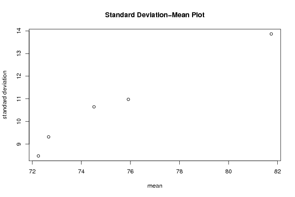
| Title produced by software | Standard Deviation-Mean Plot | ||||||||||||||||||||||||||||||||||||||||||||||||||||||||||||||||||||||||||||||||||||||||||||||||||||||||||||||||||||||||||||||||
| Date of computation | Thu, 18 Dec 2008 11:24:23 -0700 | ||||||||||||||||||||||||||||||||||||||||||||||||||||||||||||||||||||||||||||||||||||||||||||||||||||||||||||||||||||||||||||||||
| Cite this page as follows | Statistical Computations at FreeStatistics.org, Office for Research Development and Education, URL https://freestatistics.org/blog/index.php?v=date/2008/Dec/18/t12296248963oq0a47qxqjoxdy.htm/, Retrieved Sun, 12 May 2024 00:24:57 +0000 | ||||||||||||||||||||||||||||||||||||||||||||||||||||||||||||||||||||||||||||||||||||||||||||||||||||||||||||||||||||||||||||||||
| Statistical Computations at FreeStatistics.org, Office for Research Development and Education, URL https://freestatistics.org/blog/index.php?pk=34918, Retrieved Sun, 12 May 2024 00:24:57 +0000 | |||||||||||||||||||||||||||||||||||||||||||||||||||||||||||||||||||||||||||||||||||||||||||||||||||||||||||||||||||||||||||||||||
| QR Codes: | |||||||||||||||||||||||||||||||||||||||||||||||||||||||||||||||||||||||||||||||||||||||||||||||||||||||||||||||||||||||||||||||||
|
| |||||||||||||||||||||||||||||||||||||||||||||||||||||||||||||||||||||||||||||||||||||||||||||||||||||||||||||||||||||||||||||||||
| Original text written by user: | |||||||||||||||||||||||||||||||||||||||||||||||||||||||||||||||||||||||||||||||||||||||||||||||||||||||||||||||||||||||||||||||||
| IsPrivate? | No (this computation is public) | ||||||||||||||||||||||||||||||||||||||||||||||||||||||||||||||||||||||||||||||||||||||||||||||||||||||||||||||||||||||||||||||||
| User-defined keywords | |||||||||||||||||||||||||||||||||||||||||||||||||||||||||||||||||||||||||||||||||||||||||||||||||||||||||||||||||||||||||||||||||
| Estimated Impact | 189 | ||||||||||||||||||||||||||||||||||||||||||||||||||||||||||||||||||||||||||||||||||||||||||||||||||||||||||||||||||||||||||||||||
Tree of Dependent Computations | |||||||||||||||||||||||||||||||||||||||||||||||||||||||||||||||||||||||||||||||||||||||||||||||||||||||||||||||||||||||||||||||||
| Family? (F = Feedback message, R = changed R code, M = changed R Module, P = changed Parameters, D = changed Data) | |||||||||||||||||||||||||||||||||||||||||||||||||||||||||||||||||||||||||||||||||||||||||||||||||||||||||||||||||||||||||||||||||
| - [Standard Deviation-Mean Plot] [tinneke_debock.pa...] [2008-12-18 18:24:23] [20137734a2343a7bbbd59daaec7ad301] [Current] - D [Standard Deviation-Mean Plot] [tinneke_debock.pa...] [2008-12-18 18:44:03] [f9c5a49917ff87aeb076072f2749ef70] - D [Standard Deviation-Mean Plot] [Paper statistiek_...] [2008-12-19 09:21:05] [fdc296cbeb5d8064cb0dbd634c3fdc55] - D [Standard Deviation-Mean Plot] [Paper statistiek_...] [2008-12-19 09:25:10] [fdc296cbeb5d8064cb0dbd634c3fdc55] - RMPD [(Partial) Autocorrelation Function] [tinneke_debock.pa...] [2008-12-18 19:00:06] [f9c5a49917ff87aeb076072f2749ef70] - PD [(Partial) Autocorrelation Function] [Paper statistiek_...] [2008-12-19 09:30:17] [fdc296cbeb5d8064cb0dbd634c3fdc55] - D [(Partial) Autocorrelation Function] [Paper statistiek_...] [2008-12-19 09:33:45] [fdc296cbeb5d8064cb0dbd634c3fdc55] - PD [(Partial) Autocorrelation Function] [Paper statistiek_...] [2008-12-19 09:44:19] [fdc296cbeb5d8064cb0dbd634c3fdc55] - P [(Partial) Autocorrelation Function] [Paper statistiek_...] [2008-12-19 09:47:25] [fdc296cbeb5d8064cb0dbd634c3fdc55] - P [(Partial) Autocorrelation Function] [Paper statistiek_...] [2008-12-20 14:10:57] [fdc296cbeb5d8064cb0dbd634c3fdc55] - P [(Partial) Autocorrelation Function] [Paper statistiek_...] [2008-12-20 14:08:10] [fdc296cbeb5d8064cb0dbd634c3fdc55] - PD [(Partial) Autocorrelation Function] [Paper statistiek_...] [2008-12-20 14:04:23] [fdc296cbeb5d8064cb0dbd634c3fdc55] - PD [(Partial) Autocorrelation Function] [Paper statistiek_...] [2008-12-19 09:40:12] [fdc296cbeb5d8064cb0dbd634c3fdc55] - P [(Partial) Autocorrelation Function] [Paper statistiek_...] [2008-12-19 10:12:55] [fdc296cbeb5d8064cb0dbd634c3fdc55] | |||||||||||||||||||||||||||||||||||||||||||||||||||||||||||||||||||||||||||||||||||||||||||||||||||||||||||||||||||||||||||||||||
| Feedback Forum | |||||||||||||||||||||||||||||||||||||||||||||||||||||||||||||||||||||||||||||||||||||||||||||||||||||||||||||||||||||||||||||||||
Post a new message | |||||||||||||||||||||||||||||||||||||||||||||||||||||||||||||||||||||||||||||||||||||||||||||||||||||||||||||||||||||||||||||||||
Dataset | |||||||||||||||||||||||||||||||||||||||||||||||||||||||||||||||||||||||||||||||||||||||||||||||||||||||||||||||||||||||||||||||||
| Dataseries X: | |||||||||||||||||||||||||||||||||||||||||||||||||||||||||||||||||||||||||||||||||||||||||||||||||||||||||||||||||||||||||||||||||
100,8 100,7 86,2 83,2 71,7 77,5 89,8 80,3 78,7 93,8 57,6 60,6 91 85,3 77,4 77,3 68,3 69,9 81,7 75,1 69,9 84 54,3 60 89,9 77 85,3 77,6 69,2 75,5 85,7 72,2 79,9 85,3 52,2 61,2 82,4 85,4 78,2 70,2 70,2 69,3 77,5 66,1 69 79,2 56,2 63,3 77,8 92 78,1 65,1 71,1 70,9 72 81,9 70,6 72,5 65,1 54,9 80 | |||||||||||||||||||||||||||||||||||||||||||||||||||||||||||||||||||||||||||||||||||||||||||||||||||||||||||||||||||||||||||||||||
Tables (Output of Computation) | |||||||||||||||||||||||||||||||||||||||||||||||||||||||||||||||||||||||||||||||||||||||||||||||||||||||||||||||||||||||||||||||||
| |||||||||||||||||||||||||||||||||||||||||||||||||||||||||||||||||||||||||||||||||||||||||||||||||||||||||||||||||||||||||||||||||
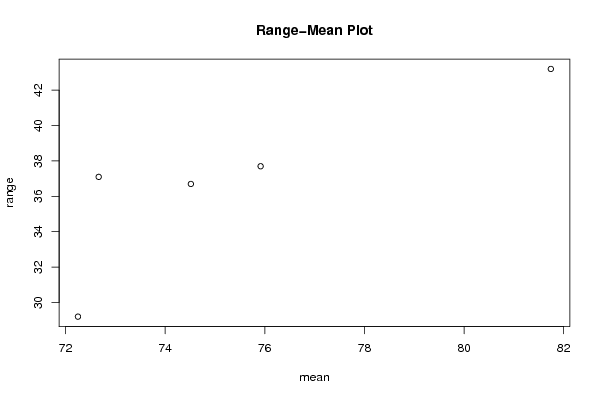
Figures (Output of Computation) | |||||||||||||||||||||||||||||||||||||||||||||||||||||||||||||||||||||||||||||||||||||||||||||||||||||||||||||||||||||||||||||||||
Input Parameters & R Code | |||||||||||||||||||||||||||||||||||||||||||||||||||||||||||||||||||||||||||||||||||||||||||||||||||||||||||||||||||||||||||||||||
| Parameters (Session): | |||||||||||||||||||||||||||||||||||||||||||||||||||||||||||||||||||||||||||||||||||||||||||||||||||||||||||||||||||||||||||||||||
| par1 = 12 ; | |||||||||||||||||||||||||||||||||||||||||||||||||||||||||||||||||||||||||||||||||||||||||||||||||||||||||||||||||||||||||||||||||
| Parameters (R input): | |||||||||||||||||||||||||||||||||||||||||||||||||||||||||||||||||||||||||||||||||||||||||||||||||||||||||||||||||||||||||||||||||
| par1 = 12 ; | |||||||||||||||||||||||||||||||||||||||||||||||||||||||||||||||||||||||||||||||||||||||||||||||||||||||||||||||||||||||||||||||||
| R code (references can be found in the software module): | |||||||||||||||||||||||||||||||||||||||||||||||||||||||||||||||||||||||||||||||||||||||||||||||||||||||||||||||||||||||||||||||||
par1 <- as.numeric(par1) | |||||||||||||||||||||||||||||||||||||||||||||||||||||||||||||||||||||||||||||||||||||||||||||||||||||||||||||||||||||||||||||||||