Free Statistics
of Irreproducible Research!
Description of Statistical Computation | |||||||||||||||||||||
|---|---|---|---|---|---|---|---|---|---|---|---|---|---|---|---|---|---|---|---|---|---|
| Author's title | |||||||||||||||||||||
| Author | *The author of this computation has been verified* | ||||||||||||||||||||
| R Software Module | rwasp_meanplot.wasp | ||||||||||||||||||||
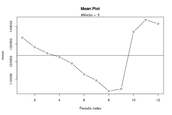
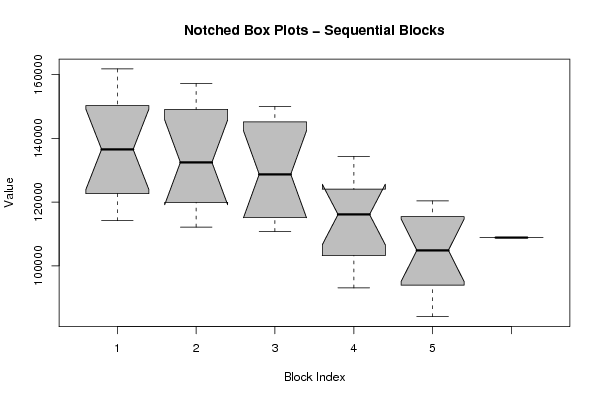
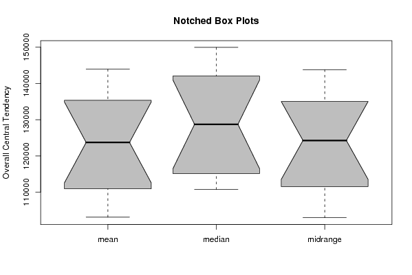
| Title produced by software | Mean Plot | ||||||||||||||||||||
| Date of computation | Thu, 18 Dec 2008 11:13:03 -0700 | ||||||||||||||||||||
| Cite this page as follows | Statistical Computations at FreeStatistics.org, Office for Research Development and Education, URL https://freestatistics.org/blog/index.php?v=date/2008/Dec/18/t1229624013qiavjcghauhbww0.htm/, Retrieved Sat, 11 May 2024 13:28:34 +0000 | ||||||||||||||||||||
| Statistical Computations at FreeStatistics.org, Office for Research Development and Education, URL https://freestatistics.org/blog/index.php?pk=34906, Retrieved Sat, 11 May 2024 13:28:34 +0000 | |||||||||||||||||||||
| QR Codes: | |||||||||||||||||||||
|
| |||||||||||||||||||||
| Original text written by user: | |||||||||||||||||||||
| IsPrivate? | No (this computation is public) | ||||||||||||||||||||
| User-defined keywords | mean plot | ||||||||||||||||||||
| Estimated Impact | 173 | ||||||||||||||||||||
Tree of Dependent Computations | |||||||||||||||||||||
| Family? (F = Feedback message, R = changed R code, M = changed R Module, P = changed Parameters, D = changed Data) | |||||||||||||||||||||
| F [Maximum-likelihood Fitting - Normal Distribution] [workshop 2 Q5 Nor...] [2008-11-13 10:44:33] [47f64d63202c1921bd27f3073f07a153] F R D [Maximum-likelihood Fitting - Normal Distribution] [Normal distribution] [2008-11-13 19:18:39] [3ffd109c9e040b1ae7e5dbe576d4698c] - RMPD [Mean Plot] [mean plot] [2008-12-10 18:47:53] [3ffd109c9e040b1ae7e5dbe576d4698c] - [Mean Plot] [mean plot] [2008-12-18 18:13:03] [962e6c9020896982bc8283b8971710a9] [Current] - [Mean Plot] [Mean plot] [2008-12-24 11:53:26] [3f66c6f083b1153972739491b89fa2dd] | |||||||||||||||||||||
| Feedback Forum | |||||||||||||||||||||
Post a new message | |||||||||||||||||||||
Dataset | |||||||||||||||||||||
| Dataseries X: | |||||||||||||||||||||
147768 137507 136919 136151 133001 125554 119647 114158 116193 152803 161761 160942 149470 139208 134588 130322 126611 122401 117352 112135 112879 148729 157230 157221 146681 136524 132111 125326 122716 116615 113719 110737 112093 143565 149946 149147 134339 122683 115614 116566 111272 104609 101802 94542 93051 124129 130374 123946 114971 105531 104919 104782 101281 94545 93248 84031 87486 115867 120327 117008 108811 | |||||||||||||||||||||
Tables (Output of Computation) | |||||||||||||||||||||
| |||||||||||||||||||||
Figures (Output of Computation) | |||||||||||||||||||||
Input Parameters & R Code | |||||||||||||||||||||
| Parameters (Session): | |||||||||||||||||||||
| par1 = 12 ; | |||||||||||||||||||||
| Parameters (R input): | |||||||||||||||||||||
| par1 = 12 ; | |||||||||||||||||||||
| R code (references can be found in the software module): | |||||||||||||||||||||
par1 <- as.numeric(par1) | |||||||||||||||||||||