Free Statistics
of Irreproducible Research!
Description of Statistical Computation | |||||||||||||||||||||||||||||||||||||||||||||
|---|---|---|---|---|---|---|---|---|---|---|---|---|---|---|---|---|---|---|---|---|---|---|---|---|---|---|---|---|---|---|---|---|---|---|---|---|---|---|---|---|---|---|---|---|---|
| Author's title | |||||||||||||||||||||||||||||||||||||||||||||
| Author | *The author of this computation has been verified* | ||||||||||||||||||||||||||||||||||||||||||||
| R Software Module | rwasp_bidensity.wasp | ||||||||||||||||||||||||||||||||||||||||||||
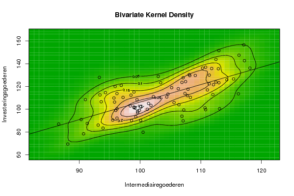
| Title produced by software | Bivariate Kernel Density Estimation | ||||||||||||||||||||||||||||||||||||||||||||
| Date of computation | Thu, 18 Dec 2008 10:08:12 -0700 | ||||||||||||||||||||||||||||||||||||||||||||
| Cite this page as follows | Statistical Computations at FreeStatistics.org, Office for Research Development and Education, URL https://freestatistics.org/blog/index.php?v=date/2008/Dec/18/t1229620125770avrvkytsssiy.htm/, Retrieved Sun, 12 May 2024 10:26:51 +0000 | ||||||||||||||||||||||||||||||||||||||||||||
| Statistical Computations at FreeStatistics.org, Office for Research Development and Education, URL https://freestatistics.org/blog/index.php?pk=34892, Retrieved Sun, 12 May 2024 10:26:51 +0000 | |||||||||||||||||||||||||||||||||||||||||||||
| QR Codes: | |||||||||||||||||||||||||||||||||||||||||||||
|
| |||||||||||||||||||||||||||||||||||||||||||||
| Original text written by user: | |||||||||||||||||||||||||||||||||||||||||||||
| IsPrivate? | No (this computation is public) | ||||||||||||||||||||||||||||||||||||||||||||
| User-defined keywords | |||||||||||||||||||||||||||||||||||||||||||||
| Estimated Impact | 153 | ||||||||||||||||||||||||||||||||||||||||||||
Tree of Dependent Computations | |||||||||||||||||||||||||||||||||||||||||||||
| Family? (F = Feedback message, R = changed R code, M = changed R Module, P = changed Parameters, D = changed Data) | |||||||||||||||||||||||||||||||||||||||||||||
| F [Univariate Data Series] [HPC Retail Sales] [2008-03-02 15:42:48] [74be16979710d4c4e7c6647856088456] - RMPD [Bivariate Kernel Density Estimation] [Paper 1] [2008-12-18 17:08:12] [0458bd763b171003ec052ce63099d477] [Current] | |||||||||||||||||||||||||||||||||||||||||||||
| Feedback Forum | |||||||||||||||||||||||||||||||||||||||||||||
Post a new message | |||||||||||||||||||||||||||||||||||||||||||||
Dataset | |||||||||||||||||||||||||||||||||||||||||||||
| Dataseries X: | |||||||||||||||||||||||||||||||||||||||||||||
90.70 94.30 104.60 111.10 110.80 107.20 99.00 99.00 91.00 96.20 96.90 96.20 100.10 99.00 115.40 106.90 107.10 99.30 99.20 108.30 105.60 99.50 107.40 93.10 88.10 110.70 113.10 99.60 93.60 98.60 99.60 114.30 107.80 101.20 112.50 100.50 93.90 116.20 112.00 106.40 95.70 96.00 95.80 103.00 102.20 98.40 111.40 86.60 91.30 107.90 101.80 104.40 93.40 100.10 98.50 112.90 101.40 107.10 110.80 90.30 95.50 111.40 113.00 107.50 95.90 106.30 105.20 117.20 106.90 108.20 113.00 97.20 99.90 108.10 118.10 109.10 93.30 112.10 111.80 112.50 116.30 110.30 117.10 103.40 96.20 | |||||||||||||||||||||||||||||||||||||||||||||
| Dataseries Y: | |||||||||||||||||||||||||||||||||||||||||||||
78.40 114.60 113.30 117.00 99.60 99.40 101.90 115.20 108.50 113.80 121.00 92.20 90.20 101.50 126.60 93.90 89.80 93.40 101.50 110.40 105.90 108.40 113.90 86.10 69.40 101.20 100.50 98.00 106.60 90.10 96.90 125.90 112.00 100.00 123.90 79.80 83.40 113.60 112.90 104.00 109.90 99.00 106.30 128.90 111.10 102.90 130.00 87.00 87.50 117.60 103.40 110.80 112.60 102.50 112.40 135.60 105.10 127.70 137.00 91.00 90.50 122.40 123.30 124.30 120.00 118.10 119.00 142.70 123.60 129.60 151.60 110.40 99.20 130.50 136.20 129.70 128.00 121.60 135.80 143.80 147.50 136.20 156.60 123.30 100.40 | |||||||||||||||||||||||||||||||||||||||||||||
Tables (Output of Computation) | |||||||||||||||||||||||||||||||||||||||||||||
| |||||||||||||||||||||||||||||||||||||||||||||
Figures (Output of Computation) | |||||||||||||||||||||||||||||||||||||||||||||
Input Parameters & R Code | |||||||||||||||||||||||||||||||||||||||||||||
| Parameters (Session): | |||||||||||||||||||||||||||||||||||||||||||||
| par1 = 50 ; par2 = 50 ; par3 = 0 ; par4 = 0 ; par5 = 0 ; par6 = Y ; par7 = Y ; | |||||||||||||||||||||||||||||||||||||||||||||
| Parameters (R input): | |||||||||||||||||||||||||||||||||||||||||||||
| par1 = 50 ; par2 = 50 ; par3 = 0 ; par4 = 0 ; par5 = 0 ; par6 = Y ; par7 = Y ; | |||||||||||||||||||||||||||||||||||||||||||||
| R code (references can be found in the software module): | |||||||||||||||||||||||||||||||||||||||||||||
par1 <- as(par1,'numeric') | |||||||||||||||||||||||||||||||||||||||||||||