Free Statistics
of Irreproducible Research!
Description of Statistical Computation | |||||||||||||||||||||
|---|---|---|---|---|---|---|---|---|---|---|---|---|---|---|---|---|---|---|---|---|---|
| Author's title | |||||||||||||||||||||
| Author | *The author of this computation has been verified* | ||||||||||||||||||||
| R Software Module | rwasp_meanplot.wasp | ||||||||||||||||||||
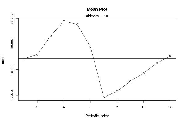
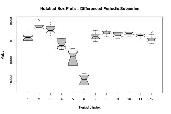
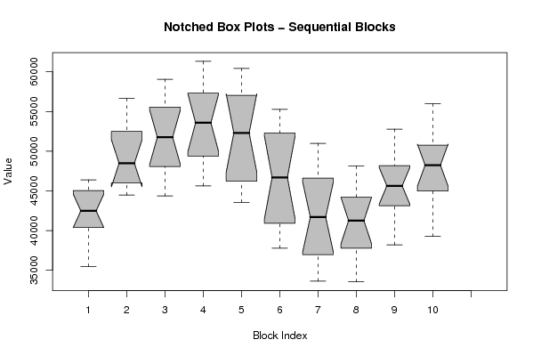
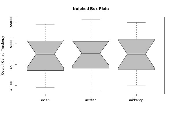
| Title produced by software | Mean Plot | ||||||||||||||||||||
| Date of computation | Thu, 18 Dec 2008 09:10:04 -0700 | ||||||||||||||||||||
| Cite this page as follows | Statistical Computations at FreeStatistics.org, Office for Research Development and Education, URL https://freestatistics.org/blog/index.php?v=date/2008/Dec/18/t1229616647j0jlz792r2d0y80.htm/, Retrieved Sun, 12 May 2024 09:36:39 +0000 | ||||||||||||||||||||
| Statistical Computations at FreeStatistics.org, Office for Research Development and Education, URL https://freestatistics.org/blog/index.php?pk=34871, Retrieved Sun, 12 May 2024 09:36:39 +0000 | |||||||||||||||||||||
| QR Codes: | |||||||||||||||||||||
|
| |||||||||||||||||||||
| Original text written by user: | |||||||||||||||||||||
| IsPrivate? | No (this computation is public) | ||||||||||||||||||||
| User-defined keywords | |||||||||||||||||||||
| Estimated Impact | 186 | ||||||||||||||||||||
Tree of Dependent Computations | |||||||||||||||||||||
| Family? (F = Feedback message, R = changed R code, M = changed R Module, P = changed Parameters, D = changed Data) | |||||||||||||||||||||
| - [(Partial) Autocorrelation Function] [(Partial) Autocor...] [2008-12-11 14:56:15] [87cabf13a90315c7085b765dcebb7412] - P [(Partial) Autocorrelation Function] [(Partial) Autocor...] [2008-12-11 15:06:01] [87cabf13a90315c7085b765dcebb7412] - PD [(Partial) Autocorrelation Function] [(Partial) Autocor...] [2008-12-11 15:23:01] [87cabf13a90315c7085b765dcebb7412] - P [(Partial) Autocorrelation Function] [(Partial) Autocor...] [2008-12-12 09:41:51] [87cabf13a90315c7085b765dcebb7412] - PD [(Partial) Autocorrelation Function] [autocorrelation 2...] [2008-12-18 15:13:35] [631938996a408f8d8cf3d9850ca0cd03] - RM D [Central Tendency] [central tendency ...] [2008-12-18 15:43:24] [631938996a408f8d8cf3d9850ca0cd03] - RM [Mean Plot] [mean plot tijdree...] [2008-12-18 16:03:30] [631938996a408f8d8cf3d9850ca0cd03] - D [Mean Plot] [mean plot tijdree...] [2008-12-18 16:10:04] [4e8974eee929007194de34cbeefcb780] [Current] | |||||||||||||||||||||
| Feedback Forum | |||||||||||||||||||||
Post a new message | |||||||||||||||||||||
Dataset | |||||||||||||||||||||
| Dataseries X: | |||||||||||||||||||||
40628 40167 43375 45610 46255 44375 35461 38096 40813 41582 44461 46390 45744 47990 51847 56641 55016 53119 44471 45200 46256 46922 48965 49447 51702 52837 56273 59070 57871 54862 44357 45264 47111 49050 50518 51824 53495 54623 58088 61321 60205 56527 45623 46127 48141 50648 52441 53661 54156 54245 58182 60436 59412 55903 43648 43555 45483 46956 49087 50433 50505 50890 53703 55276 53959 49732 37776 38437 40187 41626 42682 43647 43625 44352 49669 50986 48869 43127 33629 34948 36346 37607 38948 40274 40044 41139 45041 47433 48126 41639 33538 34742 37152 38399 41374 43363 44071 45080 48487 52140 52780 46700 38202 39915 42199 44356 46188 47883 48149 48201 51438 55796 55989 48794 39252 41414 43856 46086 48284 50101 | |||||||||||||||||||||
Tables (Output of Computation) | |||||||||||||||||||||
| |||||||||||||||||||||
Figures (Output of Computation) | |||||||||||||||||||||
Input Parameters & R Code | |||||||||||||||||||||
| Parameters (Session): | |||||||||||||||||||||
| par1 = 60 ; par2 = 1 ; par3 = 1 ; par4 = 0 ; par5 = 12 ; | |||||||||||||||||||||
| Parameters (R input): | |||||||||||||||||||||
| par1 = 12 ; | |||||||||||||||||||||
| R code (references can be found in the software module): | |||||||||||||||||||||
par1 <- as.numeric(par1) | |||||||||||||||||||||