Free Statistics
of Irreproducible Research!
Description of Statistical Computation | |||||||||||||||||||||
|---|---|---|---|---|---|---|---|---|---|---|---|---|---|---|---|---|---|---|---|---|---|
| Author's title | |||||||||||||||||||||
| Author | *The author of this computation has been verified* | ||||||||||||||||||||
| R Software Module | rwasp_meanplot.wasp | ||||||||||||||||||||
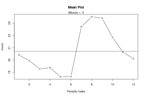
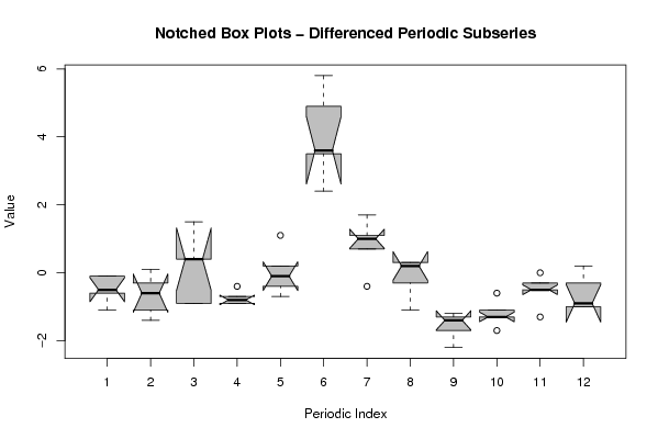
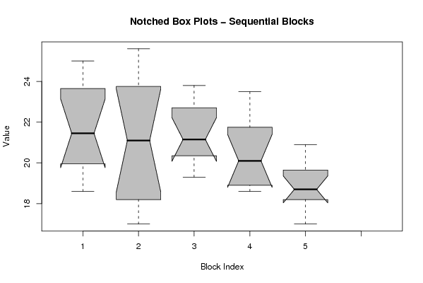
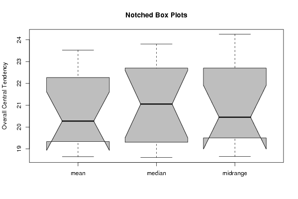
| Title produced by software | Mean Plot | ||||||||||||||||||||
| Date of computation | Thu, 18 Dec 2008 09:00:16 -0700 | ||||||||||||||||||||
| Cite this page as follows | Statistical Computations at FreeStatistics.org, Office for Research Development and Education, URL https://freestatistics.org/blog/index.php?v=date/2008/Dec/18/t1229616108ra83ffa8y2dcywo.htm/, Retrieved Sun, 12 May 2024 02:15:18 +0000 | ||||||||||||||||||||
| Statistical Computations at FreeStatistics.org, Office for Research Development and Education, URL https://freestatistics.org/blog/index.php?pk=34864, Retrieved Sun, 12 May 2024 02:15:18 +0000 | |||||||||||||||||||||
| QR Codes: | |||||||||||||||||||||
|
| |||||||||||||||||||||
| Original text written by user: | |||||||||||||||||||||
| IsPrivate? | No (this computation is public) | ||||||||||||||||||||
| User-defined keywords | |||||||||||||||||||||
| Estimated Impact | 183 | ||||||||||||||||||||
Tree of Dependent Computations | |||||||||||||||||||||
| Family? (F = Feedback message, R = changed R code, M = changed R Module, P = changed Parameters, D = changed Data) | |||||||||||||||||||||
| - [Univariate Data Series] [Werkloosheid - Jo...] [2008-12-14 16:04:23] [44ec60eb6065a3f81a5f756bd5af1faf] - RMPD [Mean Plot] [Werkloosheid - Jo...] [2008-12-18 16:00:16] [924502d03698cd41cacbcd1327858815] [Current] | |||||||||||||||||||||
| Feedback Forum | |||||||||||||||||||||
Post a new message | |||||||||||||||||||||
Dataset | |||||||||||||||||||||
| Dataseries X: | |||||||||||||||||||||
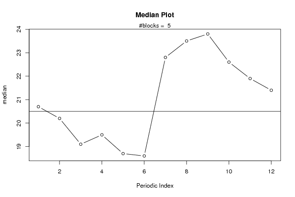
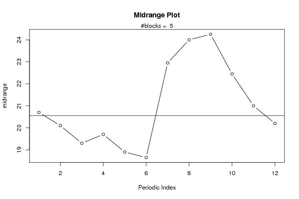
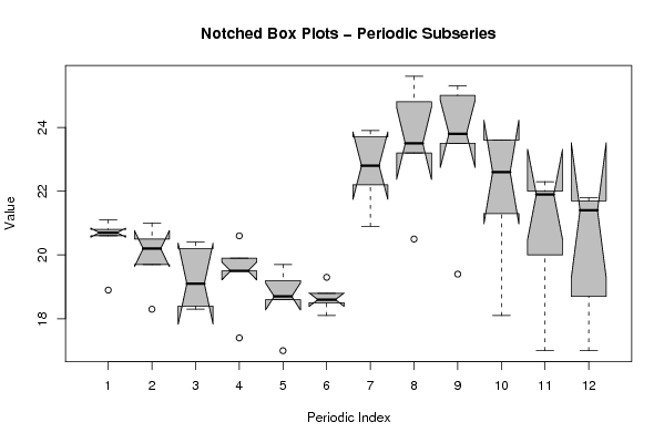
21.1 21 20.4 19.5 18.6 18.8 23.7 24.8 25 23.6 22.3 21.8 20.8 19.7 18.3 17.4 17 18.1 23.9 25.6 25.3 23.6 21.9 21.4 20.6 20.5 20.2 20.6 19.7 19.3 22.8 23.5 23.8 22.6 22 21.7 20.7 20.2 19.1 19.5 18.7 18.6 22.2 23.2 23.5 21.3 20 18.7 18.9 18.3 18.4 19.9 19.2 18.5 20.9 20.5 19.4 18.1 17 17 | |||||||||||||||||||||
Tables (Output of Computation) | |||||||||||||||||||||
| |||||||||||||||||||||
Figures (Output of Computation) | |||||||||||||||||||||
Input Parameters & R Code | |||||||||||||||||||||
| Parameters (Session): | |||||||||||||||||||||
| par1 = 12 ; | |||||||||||||||||||||
| Parameters (R input): | |||||||||||||||||||||
| par1 = 12 ; | |||||||||||||||||||||
| R code (references can be found in the software module): | |||||||||||||||||||||
par1 <- as.numeric(par1) | |||||||||||||||||||||