Repository of Reproducible Computations

Free Statistics

of Irreproducible Research!

Author's title

Author

*Unverified author*

R Software Module

rwasp_arimaforecasting.wasp

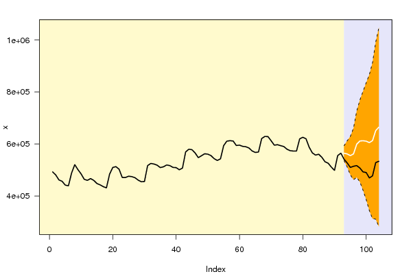
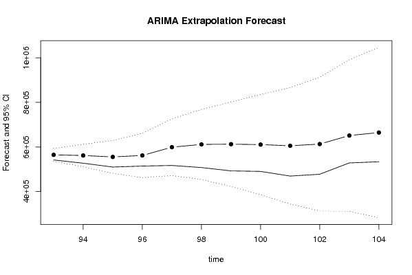
Title produced by software

ARIMA Forecasting

Date of computation

Thu, 18 Dec 2008 06:18:00 -0700

Cite this page as follows

Statistical Computations at FreeStatistics.org, Office for Research Development and Education, URL https://freestatistics.org/blog/index.php?v=date/2008/Dec/18/t1229606321frnd8un964lpo1t.htm/, Retrieved Sun, 12 May 2024 05:37:20 +0000

Statistical Computations at FreeStatistics.org, Office for Research Development and Education, URL https://freestatistics.org/blog/index.php?pk=34736, Retrieved Sun, 12 May 2024 05:37:20 +0000

QR Codes:

Paste this QR Code to cite your computation.

Original text written by user:

IsPrivate?

No (this computation is public)

User-defined keywords

Severijns Britt

Estimated Impact

165

Family? (F = Feedback message, R = changed R code, M = changed R Module, P = changed Parameters, D = changed Data)

-       [ARIMA Forecasting] [paper forcasting] [2008-12-18 13:18:00] [78308c9f3efc33d1da821bcd963df161] [Current]
- RMP     [Spectral Analysis] [paper spectraal  ...] [2008-12-18 15:08:37] [9ea94c8297ec7e569f27218c1d8ea30f] 
- RMP     [Variance Reduction Matrix] [paper variantie] [2008-12-18 15:10:32] [9ea94c8297ec7e569f27218c1d8ea30f] 
- RMP     [(Partial) Autocorrelation Function] [paper ACF d en D 0] [2008-12-18 15:12:37] [9ea94c8297ec7e569f27218c1d8ea30f] 
- RMP     [(Partial) Autocorrelation Function] [paper ACF d 1] [2008-12-18 15:14:11] [9ea94c8297ec7e569f27218c1d8ea30f] 
- RMP     [(Partial) Autocorrelation Function] [paper ACF d en D 1] [2008-12-18 15:18:32] [9ea94c8297ec7e569f27218c1d8ea30f] 
- RMP     [Spectral Analysis] [paper spectraal  ...] [2008-12-18 15:20:30] [9ea94c8297ec7e569f27218c1d8ea30f] 
- RMP     [Standard Deviation-Mean Plot] [paper lambda] [2008-12-18 15:25:35] [9ea94c8297ec7e569f27218c1d8ea30f] 
-   P     [ARIMA Forecasting] [paper forcasting 2] [2008-12-21 09:14:59] [9ea94c8297ec7e569f27218c1d8ea30f] 

Feedback Forum

Post a new message

Dataseries X:

Download CSV

Histogram

Boxplots

Summary of computational transaction
Raw Input	view raw input (R code)
Raw Output	view raw output of R engine
Computing time	2 seconds
R Server	'Sir Ronald Aylmer Fisher' @ 193.190.124.24

\begin{tabular}{lllllllll}
\hline
Summary of computational transaction \tabularnewline
Raw Input & view raw input (R code)  \tabularnewline
Raw Output & view raw output of R engine  \tabularnewline
Computing time & 2 seconds \tabularnewline
R Server & 'Sir Ronald Aylmer Fisher' @ 193.190.124.24 \tabularnewline
\hline
\end{tabular}
%Source: https://freestatistics.org/blog/index.php?pk=34736&T=0

[TABLE]
[ROW][C]Summary of computational transaction[/C][/ROW]
[ROW][C]Raw Input[/C][C]view raw input (R code) [/C][/ROW]
[ROW][C]Raw Output[/C][C]view raw output of R engine [/C][/ROW]
[ROW][C]Computing time[/C][C]2 seconds[/C][/ROW]
[ROW][C]R Server[/C][C]'Sir Ronald Aylmer Fisher' @ 193.190.124.24[/C][/ROW]
[/TABLE]
Source: https://freestatistics.org/blog/index.php?pk=34736&T=0

Globally Unique Identifier (entire table): ba.freestatistics.org/blog/index.php?pk=34736&T=0

As an alternative you can also use a QR Code:

The GUIDs for individual cells are displayed in the table below:

Summary of computational transaction
Raw Input	view raw input (R code)
Raw Output	view raw output of R engine
Computing time	2 seconds
R Server	'Sir Ronald Aylmer Fisher' @ 193.190.124.24

Univariate ARIMA Extrapolation Forecast
time	Y[t]	F[t]	95% LB	95% UB	p-value(H0: Y[t] = F[t])	P(F[t]>Y[t-1])	P(F[t]>Y[t-s])	P(F[t]>Y[92])
86	548854	-	-	-	-	-	-	-
87	531673	-	-	-	-	-	-	-
88	525919	-	-	-	-	-	-	-
89	511038	-	-	-	-	-	-	-
90	498662	-	-	-	-	-	-	-
91	555362	-	-	-	-	-	-	-
92	564591	-	-	-	-	-	-	-
93	541657	564564.7506	535858.2646	593271.2367	0.0589	0.4993	0.9876	0.4993
94	527070	561650.7153	511281.1669	612020.2638	0.0892	0.7817	0.9178	0.4545
95	509846	555206.8377	481315.2556	629098.4198	0.1144	0.7723	0.8793	0.4017
96	514258	561888.3822	462321.4977	661455.2667	0.1742	0.8472	0.8934	0.4788
97	516922	599004.8994	471651.9821	726357.8168	0.1032	0.9039	0.7491	0.7018
98	507561	611415.6313	454215.7602	768615.5024	0.0977	0.8806	0.7203	0.7203
99	492622	612459.26	422499.2773	802419.2427	0.1081	0.8604	0.7675	0.6893
100	490243	610615.1028	385864.7567	835365.4489	0.1469	0.8483	0.7669	0.6559
101	469357	605241.1033	343790.1421	866692.0645	0.1542	0.8057	0.7627	0.6197
102	477580	612992.5258	313030.0403	912955.0113	0.1881	0.826	0.7406	0.6241
103	528379	651178.9212	310978.3677	991379.4746	0.2396	0.8414	0.7804	0.6911
104	533590	664659.5311	282514.6886	1046804.3735	0.2507	0.7577	0.7898	0.6961

\begin{tabular}{lllllllll}
\hline
Univariate ARIMA Extrapolation Forecast \tabularnewline
time & Y[t] & F[t] & 95% LB & 95% UB & p-value(H0: Y[t] = F[t]) & P(F[t]>Y[t-1]) & P(F[t]>Y[t-s]) & P(F[t]>Y[92]) \tabularnewline
86 & 548854 & - & - & - & - & - & - & - \tabularnewline
87 & 531673 & - & - & - & - & - & - & - \tabularnewline
88 & 525919 & - & - & - & - & - & - & - \tabularnewline
89 & 511038 & - & - & - & - & - & - & - \tabularnewline
90 & 498662 & - & - & - & - & - & - & - \tabularnewline
91 & 555362 & - & - & - & - & - & - & - \tabularnewline
92 & 564591 & - & - & - & - & - & - & - \tabularnewline
93 & 541657 & 564564.7506 & 535858.2646 & 593271.2367 & 0.0589 & 0.4993 & 0.9876 & 0.4993 \tabularnewline
94 & 527070 & 561650.7153 & 511281.1669 & 612020.2638 & 0.0892 & 0.7817 & 0.9178 & 0.4545 \tabularnewline
95 & 509846 & 555206.8377 & 481315.2556 & 629098.4198 & 0.1144 & 0.7723 & 0.8793 & 0.4017 \tabularnewline
96 & 514258 & 561888.3822 & 462321.4977 & 661455.2667 & 0.1742 & 0.8472 & 0.8934 & 0.4788 \tabularnewline
97 & 516922 & 599004.8994 & 471651.9821 & 726357.8168 & 0.1032 & 0.9039 & 0.7491 & 0.7018 \tabularnewline
98 & 507561 & 611415.6313 & 454215.7602 & 768615.5024 & 0.0977 & 0.8806 & 0.7203 & 0.7203 \tabularnewline
99 & 492622 & 612459.26 & 422499.2773 & 802419.2427 & 0.1081 & 0.8604 & 0.7675 & 0.6893 \tabularnewline
100 & 490243 & 610615.1028 & 385864.7567 & 835365.4489 & 0.1469 & 0.8483 & 0.7669 & 0.6559 \tabularnewline
101 & 469357 & 605241.1033 & 343790.1421 & 866692.0645 & 0.1542 & 0.8057 & 0.7627 & 0.6197 \tabularnewline
102 & 477580 & 612992.5258 & 313030.0403 & 912955.0113 & 0.1881 & 0.826 & 0.7406 & 0.6241 \tabularnewline
103 & 528379 & 651178.9212 & 310978.3677 & 991379.4746 & 0.2396 & 0.8414 & 0.7804 & 0.6911 \tabularnewline
104 & 533590 & 664659.5311 & 282514.6886 & 1046804.3735 & 0.2507 & 0.7577 & 0.7898 & 0.6961 \tabularnewline
\hline
\end{tabular}
%Source: https://freestatistics.org/blog/index.php?pk=34736&T=1

[TABLE]
[ROW][C]Univariate ARIMA Extrapolation Forecast[/C][/ROW]
[ROW][C]time[/C][C]Y[t][/C][C]F[t][/C][C]95% LB[/C][C]95% UB[/C][C]p-value(H0: Y[t] = F[t])[/C][C]P(F[t]>Y[t-1])[/C][C]P(F[t]>Y[t-s])[/C][C]P(F[t]>Y[92])[/C][/ROW]
[ROW][C]86[/C][C]548854[/C][C]-[/C][C]-[/C][C]-[/C][C]-[/C][C]-[/C][C]-[/C][C]-[/C][/ROW]
[ROW][C]87[/C][C]531673[/C][C]-[/C][C]-[/C][C]-[/C][C]-[/C][C]-[/C][C]-[/C][C]-[/C][/ROW]
[ROW][C]88[/C][C]525919[/C][C]-[/C][C]-[/C][C]-[/C][C]-[/C][C]-[/C][C]-[/C][C]-[/C][/ROW]
[ROW][C]89[/C][C]511038[/C][C]-[/C][C]-[/C][C]-[/C][C]-[/C][C]-[/C][C]-[/C][C]-[/C][/ROW]
[ROW][C]90[/C][C]498662[/C][C]-[/C][C]-[/C][C]-[/C][C]-[/C][C]-[/C][C]-[/C][C]-[/C][/ROW]
[ROW][C]91[/C][C]555362[/C][C]-[/C][C]-[/C][C]-[/C][C]-[/C][C]-[/C][C]-[/C][C]-[/C][/ROW]
[ROW][C]92[/C][C]564591[/C][C]-[/C][C]-[/C][C]-[/C][C]-[/C][C]-[/C][C]-[/C][C]-[/C][/ROW]
[ROW][C]93[/C][C]541657[/C][C]564564.7506[/C][C]535858.2646[/C][C]593271.2367[/C][C]0.0589[/C][C]0.4993[/C][C]0.9876[/C][C]0.4993[/C][/ROW]
[ROW][C]94[/C][C]527070[/C][C]561650.7153[/C][C]511281.1669[/C][C]612020.2638[/C][C]0.0892[/C][C]0.7817[/C][C]0.9178[/C][C]0.4545[/C][/ROW]
[ROW][C]95[/C][C]509846[/C][C]555206.8377[/C][C]481315.2556[/C][C]629098.4198[/C][C]0.1144[/C][C]0.7723[/C][C]0.8793[/C][C]0.4017[/C][/ROW]
[ROW][C]96[/C][C]514258[/C][C]561888.3822[/C][C]462321.4977[/C][C]661455.2667[/C][C]0.1742[/C][C]0.8472[/C][C]0.8934[/C][C]0.4788[/C][/ROW]
[ROW][C]97[/C][C]516922[/C][C]599004.8994[/C][C]471651.9821[/C][C]726357.8168[/C][C]0.1032[/C][C]0.9039[/C][C]0.7491[/C][C]0.7018[/C][/ROW]
[ROW][C]98[/C][C]507561[/C][C]611415.6313[/C][C]454215.7602[/C][C]768615.5024[/C][C]0.0977[/C][C]0.8806[/C][C]0.7203[/C][C]0.7203[/C][/ROW]
[ROW][C]99[/C][C]492622[/C][C]612459.26[/C][C]422499.2773[/C][C]802419.2427[/C][C]0.1081[/C][C]0.8604[/C][C]0.7675[/C][C]0.6893[/C][/ROW]
[ROW][C]100[/C][C]490243[/C][C]610615.1028[/C][C]385864.7567[/C][C]835365.4489[/C][C]0.1469[/C][C]0.8483[/C][C]0.7669[/C][C]0.6559[/C][/ROW]
[ROW][C]101[/C][C]469357[/C][C]605241.1033[/C][C]343790.1421[/C][C]866692.0645[/C][C]0.1542[/C][C]0.8057[/C][C]0.7627[/C][C]0.6197[/C][/ROW]
[ROW][C]102[/C][C]477580[/C][C]612992.5258[/C][C]313030.0403[/C][C]912955.0113[/C][C]0.1881[/C][C]0.826[/C][C]0.7406[/C][C]0.6241[/C][/ROW]
[ROW][C]103[/C][C]528379[/C][C]651178.9212[/C][C]310978.3677[/C][C]991379.4746[/C][C]0.2396[/C][C]0.8414[/C][C]0.7804[/C][C]0.6911[/C][/ROW]
[ROW][C]104[/C][C]533590[/C][C]664659.5311[/C][C]282514.6886[/C][C]1046804.3735[/C][C]0.2507[/C][C]0.7577[/C][C]0.7898[/C][C]0.6961[/C][/ROW]
[/TABLE]
Source: https://freestatistics.org/blog/index.php?pk=34736&T=1

Globally Unique Identifier (entire table): ba.freestatistics.org/blog/index.php?pk=34736&T=1

As an alternative you can also use a QR Code:

The GUIDs for individual cells are displayed in the table below:

Univariate ARIMA Extrapolation Forecast
time	Y[t]	F[t]	95% LB	95% UB	p-value(H0: Y[t] = F[t])	P(F[t]>Y[t-1])	P(F[t]>Y[t-s])	P(F[t]>Y[92])
86	548854	-	-	-	-	-	-	-
87	531673	-	-	-	-	-	-	-
88	525919	-	-	-	-	-	-	-
89	511038	-	-	-	-	-	-	-
90	498662	-	-	-	-	-	-	-
91	555362	-	-	-	-	-	-	-
92	564591	-	-	-	-	-	-	-
93	541657	564564.7506	535858.2646	593271.2367	0.0589	0.4993	0.9876	0.4993
94	527070	561650.7153	511281.1669	612020.2638	0.0892	0.7817	0.9178	0.4545
95	509846	555206.8377	481315.2556	629098.4198	0.1144	0.7723	0.8793	0.4017
96	514258	561888.3822	462321.4977	661455.2667	0.1742	0.8472	0.8934	0.4788
97	516922	599004.8994	471651.9821	726357.8168	0.1032	0.9039	0.7491	0.7018
98	507561	611415.6313	454215.7602	768615.5024	0.0977	0.8806	0.7203	0.7203
99	492622	612459.26	422499.2773	802419.2427	0.1081	0.8604	0.7675	0.6893
100	490243	610615.1028	385864.7567	835365.4489	0.1469	0.8483	0.7669	0.6559
101	469357	605241.1033	343790.1421	866692.0645	0.1542	0.8057	0.7627	0.6197
102	477580	612992.5258	313030.0403	912955.0113	0.1881	0.826	0.7406	0.6241
103	528379	651178.9212	310978.3677	991379.4746	0.2396	0.8414	0.7804	0.6911
104	533590	664659.5311	282514.6886	1046804.3735	0.2507	0.7577	0.7898	0.6961

Univariate ARIMA Extrapolation Forecast Performance
time	% S.E.	PE	MAPE	Sq.E	MSE	RMSE
93	0.0259	-0.0406	0.0034	524765039.5379	43730419.9615	6612.898
94	0.0458	-0.0616	0.0051	1195825873.4193	99652156.1183	9982.5927
95	0.0679	-0.0817	0.0068	2057605600.7784	171467133.3982	13094.5459
96	0.0904	-0.0848	0.0071	2268653309.3164	189054442.443	13749.707
97	0.1085	-0.137	0.0114	6737602381.2472	561466865.1039	23695.292
98	0.1312	-0.1699	0.0142	10785784437.264	898815369.772	29980.2497
99	0.1582	-0.1957	0.0163	14360968885.6223	1196747407.1352	34594.0372
100	0.1878	-0.1971	0.0164	14489443129.8896	1207453594.1575	34748.433
101	0.2204	-0.2245	0.0187	18464489524.149	1538707460.3458	39226.3618
102	0.2497	-0.2209	0.0184	18336552152.1897	1528046012.6825	39090.2291
103	0.2665	-0.1886	0.0157	15079820635.7752	1256651719.6479	35449.2838
104	0.2933	-0.1972	0.0164	17179221975.6583	1431601831.3049	37836.5145

\begin{tabular}{lllllllll}
\hline
Univariate ARIMA Extrapolation Forecast Performance \tabularnewline
time & % S.E. & PE & MAPE & Sq.E & MSE & RMSE \tabularnewline
93 & 0.0259 & -0.0406 & 0.0034 & 524765039.5379 & 43730419.9615 & 6612.898 \tabularnewline
94 & 0.0458 & -0.0616 & 0.0051 & 1195825873.4193 & 99652156.1183 & 9982.5927 \tabularnewline
95 & 0.0679 & -0.0817 & 0.0068 & 2057605600.7784 & 171467133.3982 & 13094.5459 \tabularnewline
96 & 0.0904 & -0.0848 & 0.0071 & 2268653309.3164 & 189054442.443 & 13749.707 \tabularnewline
97 & 0.1085 & -0.137 & 0.0114 & 6737602381.2472 & 561466865.1039 & 23695.292 \tabularnewline
98 & 0.1312 & -0.1699 & 0.0142 & 10785784437.264 & 898815369.772 & 29980.2497 \tabularnewline
99 & 0.1582 & -0.1957 & 0.0163 & 14360968885.6223 & 1196747407.1352 & 34594.0372 \tabularnewline
100 & 0.1878 & -0.1971 & 0.0164 & 14489443129.8896 & 1207453594.1575 & 34748.433 \tabularnewline
101 & 0.2204 & -0.2245 & 0.0187 & 18464489524.149 & 1538707460.3458 & 39226.3618 \tabularnewline
102 & 0.2497 & -0.2209 & 0.0184 & 18336552152.1897 & 1528046012.6825 & 39090.2291 \tabularnewline
103 & 0.2665 & -0.1886 & 0.0157 & 15079820635.7752 & 1256651719.6479 & 35449.2838 \tabularnewline
104 & 0.2933 & -0.1972 & 0.0164 & 17179221975.6583 & 1431601831.3049 & 37836.5145 \tabularnewline
\hline
\end{tabular}
%Source: https://freestatistics.org/blog/index.php?pk=34736&T=2

[TABLE]
[ROW][C]Univariate ARIMA Extrapolation Forecast Performance[/C][/ROW]
[ROW][C]time[/C][C]% S.E.[/C][C]PE[/C][C]MAPE[/C][C]Sq.E[/C][C]MSE[/C][C]RMSE[/C][/ROW]
[ROW][C]93[/C][C]0.0259[/C][C]-0.0406[/C][C]0.0034[/C][C]524765039.5379[/C][C]43730419.9615[/C][C]6612.898[/C][/ROW]
[ROW][C]94[/C][C]0.0458[/C][C]-0.0616[/C][C]0.0051[/C][C]1195825873.4193[/C][C]99652156.1183[/C][C]9982.5927[/C][/ROW]
[ROW][C]95[/C][C]0.0679[/C][C]-0.0817[/C][C]0.0068[/C][C]2057605600.7784[/C][C]171467133.3982[/C][C]13094.5459[/C][/ROW]
[ROW][C]96[/C][C]0.0904[/C][C]-0.0848[/C][C]0.0071[/C][C]2268653309.3164[/C][C]189054442.443[/C][C]13749.707[/C][/ROW]
[ROW][C]97[/C][C]0.1085[/C][C]-0.137[/C][C]0.0114[/C][C]6737602381.2472[/C][C]561466865.1039[/C][C]23695.292[/C][/ROW]
[ROW][C]98[/C][C]0.1312[/C][C]-0.1699[/C][C]0.0142[/C][C]10785784437.264[/C][C]898815369.772[/C][C]29980.2497[/C][/ROW]
[ROW][C]99[/C][C]0.1582[/C][C]-0.1957[/C][C]0.0163[/C][C]14360968885.6223[/C][C]1196747407.1352[/C][C]34594.0372[/C][/ROW]
[ROW][C]100[/C][C]0.1878[/C][C]-0.1971[/C][C]0.0164[/C][C]14489443129.8896[/C][C]1207453594.1575[/C][C]34748.433[/C][/ROW]
[ROW][C]101[/C][C]0.2204[/C][C]-0.2245[/C][C]0.0187[/C][C]18464489524.149[/C][C]1538707460.3458[/C][C]39226.3618[/C][/ROW]
[ROW][C]102[/C][C]0.2497[/C][C]-0.2209[/C][C]0.0184[/C][C]18336552152.1897[/C][C]1528046012.6825[/C][C]39090.2291[/C][/ROW]
[ROW][C]103[/C][C]0.2665[/C][C]-0.1886[/C][C]0.0157[/C][C]15079820635.7752[/C][C]1256651719.6479[/C][C]35449.2838[/C][/ROW]
[ROW][C]104[/C][C]0.2933[/C][C]-0.1972[/C][C]0.0164[/C][C]17179221975.6583[/C][C]1431601831.3049[/C][C]37836.5145[/C][/ROW]
[/TABLE]
Source: https://freestatistics.org/blog/index.php?pk=34736&T=2

Globally Unique Identifier (entire table): ba.freestatistics.org/blog/index.php?pk=34736&T=2

As an alternative you can also use a QR Code:

The GUIDs for individual cells are displayed in the table below:

Univariate ARIMA Extrapolation Forecast Performance
time	% S.E.	PE	MAPE	Sq.E	MSE	RMSE
93	0.0259	-0.0406	0.0034	524765039.5379	43730419.9615	6612.898
94	0.0458	-0.0616	0.0051	1195825873.4193	99652156.1183	9982.5927
95	0.0679	-0.0817	0.0068	2057605600.7784	171467133.3982	13094.5459
96	0.0904	-0.0848	0.0071	2268653309.3164	189054442.443	13749.707
97	0.1085	-0.137	0.0114	6737602381.2472	561466865.1039	23695.292
98	0.1312	-0.1699	0.0142	10785784437.264	898815369.772	29980.2497
99	0.1582	-0.1957	0.0163	14360968885.6223	1196747407.1352	34594.0372
100	0.1878	-0.1971	0.0164	14489443129.8896	1207453594.1575	34748.433
101	0.2204	-0.2245	0.0187	18464489524.149	1538707460.3458	39226.3618
102	0.2497	-0.2209	0.0184	18336552152.1897	1528046012.6825	39090.2291
103	0.2665	-0.1886	0.0157	15079820635.7752	1256651719.6479	35449.2838
104	0.2933	-0.1972	0.0164	17179221975.6583	1431601831.3049	37836.5145

Figure 1

PNG link

Postscript link

PDF link

Figure 2

PNG link

Postscript link

PDF link

Parameters (Session):

par1 = 12 ; par2 = 1 ; par3 = 2 ; par4 = 1 ; par5 = 6 ; par6 = 0 ; par7 = 1 ; par8 = 0 ; par9 = 1 ; par10 = FALSE ;

Parameters (R input):

par1 = 12 ; par2 = 1 ; par3 = 2 ; par4 = 1 ; par5 = 6 ; par6 = 0 ; par7 = 1 ; par8 = 0 ; par9 = 1 ; par10 = FALSE ;

R code (references can be found in the software module):

par1 <- as.numeric(par1) #cut off periods
par2 <- as.numeric(par2) #lambda
par3 <- as.numeric(par3) #degree of non-seasonal differencing
par4 <- as.numeric(par4) #degree of seasonal differencing
par5 <- as.numeric(par5) #seasonal period
par6 <- as.numeric(par6) #p
par7 <- as.numeric(par7) #q
par8 <- as.numeric(par8) #P
par9 <- as.numeric(par9) #Q
if (par10 == 'TRUE') par10 <- TRUE
if (par10 == 'FALSE') par10 <- FALSE
if (par2 == 0) x <- log(x)
if (par2 != 0) x <- x^par2
lx <- length(x)
first <- lx - 2*par1
nx <- lx - par1
nx1 <- nx + 1
fx <- lx - nx
if (fx < 1) {
fx <- par5
nx1 <- lx + fx - 1
first <- lx - 2*fx
}
first <- 1
if (fx < 3) fx <- round(lx/10,0)
(arima.out <- arima(x[1:nx], order=c(par6,par3,par7), seasonal=list(order=c(par8,par4,par9), period=par5), include.mean=par10, method='ML'))
(forecast <- predict(arima.out,fx))
(lb <- forecast$pred - 1.96 * forecast$se)
(ub <- forecast$pred + 1.96 * forecast$se)
if (par2 == 0) {
x <- exp(x)
forecast$pred <- exp(forecast$pred)
lb <- exp(lb)
ub <- exp(ub)
}
if (par2 != 0) {
x <- x^(1/par2)
forecast$pred <- forecast$pred^(1/par2)
lb <- lb^(1/par2)
ub <- ub^(1/par2)
}
if (par2 < 0) {
olb <- lb
lb <- ub
ub <- olb
}
(actandfor <- c(x[1:nx], forecast$pred))
(perc.se <- (ub-forecast$pred)/1.96/forecast$pred)
bitmap(file='test1.png')
opar <- par(mar=c(4,4,2,2),las=1)
ylim <- c( min(x[first:nx],lb), max(x[first:nx],ub))
plot(x,ylim=ylim,type='n',xlim=c(first,lx))
usr <- par('usr')
rect(usr[1],usr[3],nx+1,usr[4],border=NA,col='lemonchiffon')
rect(nx1,usr[3],usr[2],usr[4],border=NA,col='lavender')
abline(h= (-3:3)*2 , col ='gray', lty =3)
polygon( c(nx1:lx,lx:nx1), c(lb,rev(ub)), col = 'orange', lty=2,border=NA)
lines(nx1:lx, lb , lty=2)
lines(nx1:lx, ub , lty=2)
lines(x, lwd=2)
lines(nx1:lx, forecast$pred , lwd=2 , col ='white')
box()
par(opar)
dev.off()
prob.dec <- array(NA, dim=fx)
prob.sdec <- array(NA, dim=fx)
prob.ldec <- array(NA, dim=fx)
prob.pval <- array(NA, dim=fx)
perf.pe <- array(0, dim=fx)
perf.mape <- array(0, dim=fx)
perf.se <- array(0, dim=fx)
perf.mse <- array(0, dim=fx)
perf.rmse <- array(0, dim=fx)
for (i in 1:fx) {
locSD <- (ub[i] - forecast$pred[i]) / 1.96
perf.pe[i] = (x[nx+i] - forecast$pred[i]) / forecast$pred[i]
perf.mape[i] = perf.mape[i] + abs(perf.pe[i])
perf.se[i] = (x[nx+i] - forecast$pred[i])^2
perf.mse[i] = perf.mse[i] + perf.se[i]
prob.dec[i] = pnorm((x[nx+i-1] - forecast$pred[i]) / locSD)
prob.sdec[i] = pnorm((x[nx+i-par5] - forecast$pred[i]) / locSD)
prob.ldec[i] = pnorm((x[nx] - forecast$pred[i]) / locSD)
prob.pval[i] = pnorm(abs(x[nx+i] - forecast$pred[i]) / locSD)
}
perf.mape = perf.mape / fx
perf.mse = perf.mse / fx
perf.rmse = sqrt(perf.mse)
bitmap(file='test2.png')
plot(forecast$pred, pch=19, type='b',main='ARIMA Extrapolation Forecast', ylab='Forecast and 95% CI', xlab='time',ylim=c(min(lb),max(ub)))
dum <- forecast$pred
dum[1:12] <- x[(nx+1):lx]
lines(dum, lty=1)
lines(ub,lty=3)
lines(lb,lty=3)
dev.off()
load(file='createtable')
a<-table.start()
a<-table.row.start(a)
a<-table.element(a,'Univariate ARIMA Extrapolation Forecast',9,TRUE)
a<-table.row.end(a)
a<-table.row.start(a)
a<-table.element(a,'time',1,header=TRUE)
a<-table.element(a,'Y[t]',1,header=TRUE)
a<-table.element(a,'F[t]',1,header=TRUE)
a<-table.element(a,'95% LB',1,header=TRUE)
a<-table.element(a,'95% UB',1,header=TRUE)
a<-table.element(a,'p-value
(H0: Y[t] = F[t])',1,header=TRUE)
a<-table.element(a,'P(F[t]>Y[t-1])',1,header=TRUE)
a<-table.element(a,'P(F[t]>Y[t-s])',1,header=TRUE)
mylab <- paste('P(F[t]>Y[',nx,sep='')
mylab <- paste(mylab,'])',sep='')
a<-table.element(a,mylab,1,header=TRUE)
a<-table.row.end(a)
for (i in (nx-par5):nx) {
a<-table.row.start(a)
a<-table.element(a,i,header=TRUE)
a<-table.element(a,x[i])
a<-table.element(a,'-')
a<-table.element(a,'-')
a<-table.element(a,'-')
a<-table.element(a,'-')
a<-table.element(a,'-')
a<-table.element(a,'-')
a<-table.element(a,'-')
a<-table.row.end(a)
}
for (i in 1:fx) {
a<-table.row.start(a)
a<-table.element(a,nx+i,header=TRUE)
a<-table.element(a,round(x[nx+i],4))
a<-table.element(a,round(forecast$pred[i],4))
a<-table.element(a,round(lb[i],4))
a<-table.element(a,round(ub[i],4))
a<-table.element(a,round((1-prob.pval[i]),4))
a<-table.element(a,round((1-prob.dec[i]),4))
a<-table.element(a,round((1-prob.sdec[i]),4))
a<-table.element(a,round((1-prob.ldec[i]),4))
a<-table.row.end(a)
}
a<-table.end(a)
table.save(a,file='mytable.tab')
a<-table.start()
a<-table.row.start(a)
a<-table.element(a,'Univariate ARIMA Extrapolation Forecast Performance',7,TRUE)
a<-table.row.end(a)
a<-table.row.start(a)
a<-table.element(a,'time',1,header=TRUE)
a<-table.element(a,'% S.E.',1,header=TRUE)
a<-table.element(a,'PE',1,header=TRUE)
a<-table.element(a,'MAPE',1,header=TRUE)
a<-table.element(a,'Sq.E',1,header=TRUE)
a<-table.element(a,'MSE',1,header=TRUE)
a<-table.element(a,'RMSE',1,header=TRUE)
a<-table.row.end(a)
for (i in 1:fx) {
a<-table.row.start(a)
a<-table.element(a,nx+i,header=TRUE)
a<-table.element(a,round(perc.se[i],4))
a<-table.element(a,round(perf.pe[i],4))
a<-table.element(a,round(perf.mape[i],4))
a<-table.element(a,round(perf.se[i],4))
a<-table.element(a,round(perf.mse[i],4))
a<-table.element(a,round(perf.rmse[i],4))
a<-table.row.end(a)
}
a<-table.end(a)
table.save(a,file='mytable1.tab')

Free Statistics

Description of Statistical Computation

Tree of Dependent Computations

Dataset

Tables (Output of Computation)

Figures (Output of Computation)

Input Parameters & R Code