Free Statistics
of Irreproducible Research!
Description of Statistical Computation | |||||||||||||||||||||
|---|---|---|---|---|---|---|---|---|---|---|---|---|---|---|---|---|---|---|---|---|---|
| Author's title | |||||||||||||||||||||
| Author | *The author of this computation has been verified* | ||||||||||||||||||||
| R Software Module | rwasp_cloud.wasp | ||||||||||||||||||||
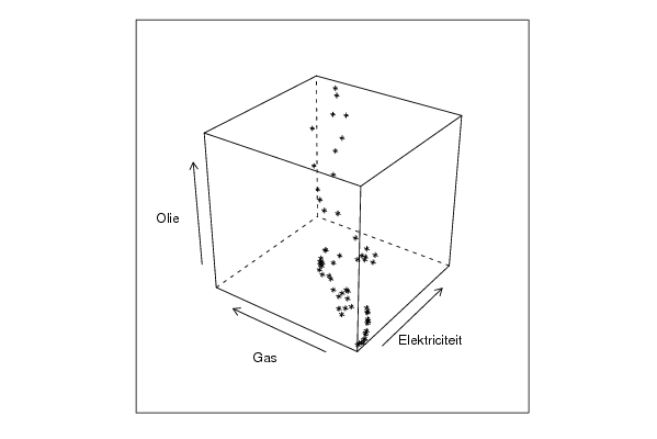
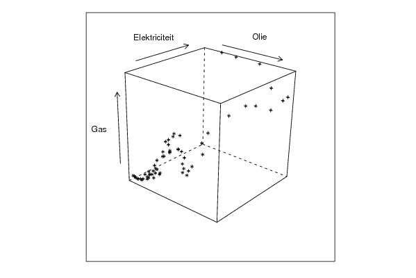
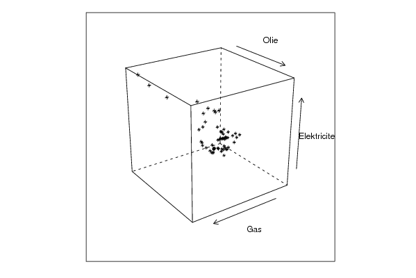
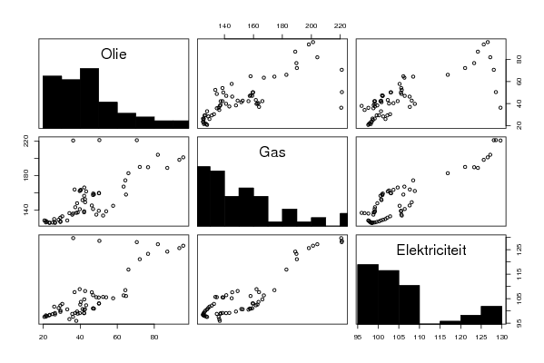
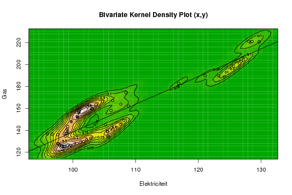
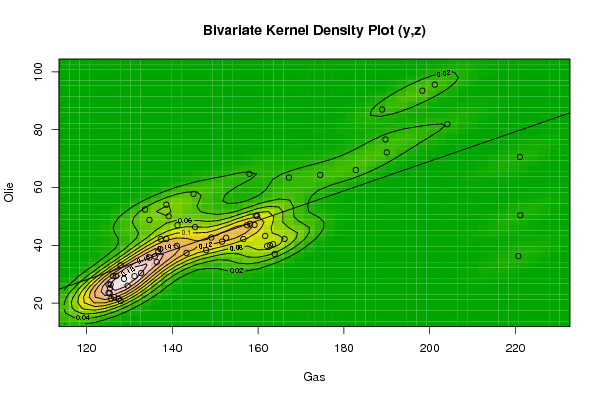
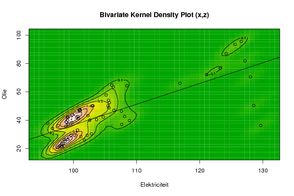
| Title produced by software | Trivariate Scatterplots | ||||||||||||||||||||
| Date of computation | Thu, 18 Dec 2008 05:45:10 -0700 | ||||||||||||||||||||
| Cite this page as follows | Statistical Computations at FreeStatistics.org, Office for Research Development and Education, URL https://freestatistics.org/blog/index.php?v=date/2008/Dec/18/t12296043626b113n91ajbl0tg.htm/, Retrieved Sun, 12 May 2024 04:38:11 +0000 | ||||||||||||||||||||
| Statistical Computations at FreeStatistics.org, Office for Research Development and Education, URL https://freestatistics.org/blog/index.php?pk=34720, Retrieved Sun, 12 May 2024 04:38:11 +0000 | |||||||||||||||||||||
| QR Codes: | |||||||||||||||||||||
|
| |||||||||||||||||||||
| Original text written by user: | |||||||||||||||||||||
| IsPrivate? | No (this computation is public) | ||||||||||||||||||||
| User-defined keywords | |||||||||||||||||||||
| Estimated Impact | 131 | ||||||||||||||||||||
Tree of Dependent Computations | |||||||||||||||||||||
| Family? (F = Feedback message, R = changed R code, M = changed R Module, P = changed Parameters, D = changed Data) | |||||||||||||||||||||
| - [Univariate Explorative Data Analysis] [Paper - Un. EDA -...] [2008-12-18 11:54:57] [85841a4a203c2f9589565c024425a91b] - RMPD [Trivariate Scatterplots] [Paper - Trivariat...] [2008-12-18 12:45:10] [07b7cf1321bc38017c2c7efcf91ca696] [Current] | |||||||||||||||||||||
| Feedback Forum | |||||||||||||||||||||
Post a new message | |||||||||||||||||||||
Dataset | |||||||||||||||||||||
| Dataseries X: | |||||||||||||||||||||
97.57 97.74 97.92 98.19 98.23 98.41 98.59 98.71 99.14 99.62 100.18 100.66 101.19 101.75 102.2 102.87 98.81 97.6 96.68 95.96 98.89 99.05 99.2 99.11 99.19 99.77 100.70 100.78 100.53 101.01 100.92 101.10 103.11 102.99 102.31 102.61 103.68 104.72 107.66 108.87 108.12 107.61 106.42 105.61 105.71 105.49 105.57 105.18 106.09 106.34 108.47 116.87 121.08 123.27 124.18 125.60 126.57 127.18 128.04 128.55 129.67 | |||||||||||||||||||||
| Dataseries Y: | |||||||||||||||||||||
127.96 127.47 126.47 125.75 125.42 125.14 125.15 125.51 125.63 126.22 126.88 127.96 128.74 129.6 131.2 132.72 134.67 135.94 136.39 136.74 137.2 137.36 138.63 141.07 143.32 147.91 152.56 151.61 156.56 157.45 158.13 159.18 159.47 159.79 161.65 162.77 163.48 166.16 163.86 162.12 149.08 145.32 141.21 134.68 133.65 139.17 138.61 144.96 157.99 167.18 174.48 182.77 190.00 189.70 188.90 198.28 201.18 204.14 221.02 221.12 220.68 | |||||||||||||||||||||
| Dataseries Z: | |||||||||||||||||||||
20.72 21.45 22.09 21.53 23.35 23.57 26.42 25.21 26.44 29.34 29.40 33.05 28.38 26.01 29.31 30.36 35.75 36.15 34.21 37.91 38.70 42.12 42.16 39.80 37.36 38.35 42.60 41.25 42.16 46.94 47.43 47.06 50.18 50.13 43.23 40.04 40.37 42.21 37.00 39.74 42.68 46.29 46.97 48.73 52.37 50.05 54.04 57.78 64.72 63.41 64.36 66.03 72.14 76.60 86.97 93.48 95.59 81.89 70.55 50.38 36.25 | |||||||||||||||||||||
Tables (Output of Computation) | |||||||||||||||||||||
| |||||||||||||||||||||
Figures (Output of Computation) | |||||||||||||||||||||
Input Parameters & R Code | |||||||||||||||||||||
| Parameters (Session): | |||||||||||||||||||||
| Parameters (R input): | |||||||||||||||||||||
| par1 = 50 ; par2 = 50 ; par3 = Y ; par4 = Y ; par5 = Elektriciteit ; par6 = Gas ; par7 = Olie ; | |||||||||||||||||||||
| R code (references can be found in the software module): | |||||||||||||||||||||
x <- array(x,dim=c(length(x),1)) | |||||||||||||||||||||