Free Statistics
of Irreproducible Research!
Description of Statistical Computation | |||||||||||||||||||||
|---|---|---|---|---|---|---|---|---|---|---|---|---|---|---|---|---|---|---|---|---|---|
| Author's title | |||||||||||||||||||||
| Author | *The author of this computation has been verified* | ||||||||||||||||||||
| R Software Module | rwasp_meanplot.wasp | ||||||||||||||||||||
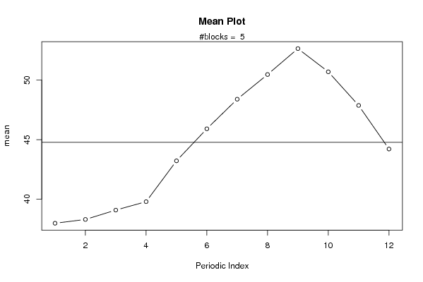
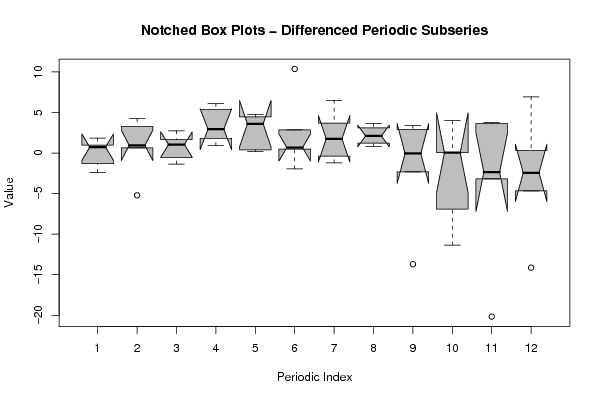
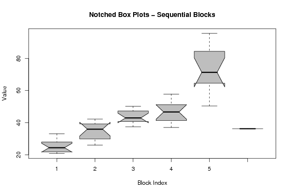
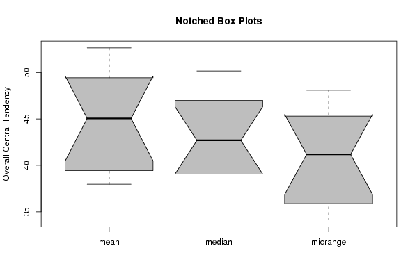
| Title produced by software | Mean Plot | ||||||||||||||||||||
| Date of computation | Thu, 18 Dec 2008 04:43:00 -0700 | ||||||||||||||||||||
| Cite this page as follows | Statistical Computations at FreeStatistics.org, Office for Research Development and Education, URL https://freestatistics.org/blog/index.php?v=date/2008/Dec/18/t12296006563vb97n5ztljwuqr.htm/, Retrieved Sat, 11 May 2024 08:46:49 +0000 | ||||||||||||||||||||
| Statistical Computations at FreeStatistics.org, Office for Research Development and Education, URL https://freestatistics.org/blog/index.php?pk=34671, Retrieved Sat, 11 May 2024 08:46:49 +0000 | |||||||||||||||||||||
| QR Codes: | |||||||||||||||||||||
|
| |||||||||||||||||||||
| Original text written by user: | |||||||||||||||||||||
| IsPrivate? | No (this computation is public) | ||||||||||||||||||||
| User-defined keywords | |||||||||||||||||||||
| Estimated Impact | 147 | ||||||||||||||||||||
Tree of Dependent Computations | |||||||||||||||||||||
| Family? (F = Feedback message, R = changed R code, M = changed R Module, P = changed Parameters, D = changed Data) | |||||||||||||||||||||
| - [Mean Plot] [Paper - Mean plot...] [2008-12-18 11:43:00] [07b7cf1321bc38017c2c7efcf91ca696] [Current] - RMP [Standard Deviation-Mean Plot] [Paper - Standard ...] [2008-12-21 17:50:16] [85841a4a203c2f9589565c024425a91b] - RMPD [Standard Deviation-Mean Plot] [Paper - Standard ...] [2008-12-21 18:00:45] [85841a4a203c2f9589565c024425a91b] - [Standard Deviation-Mean Plot] [Paper - Standard ...] [2008-12-21 18:04:34] [85841a4a203c2f9589565c024425a91b] | |||||||||||||||||||||
| Feedback Forum | |||||||||||||||||||||
Post a new message | |||||||||||||||||||||
Dataset | |||||||||||||||||||||
| Dataseries X: | |||||||||||||||||||||
20.72 21.45 22.09 21.53 23.35 23.57 26.42 25.21 26.44 29.34 29.40 33.05 28.38 26.01 29.31 30.36 35.75 36.15 34.21 37.91 38.70 42.12 42.16 39.80 37.36 38.35 42.60 41.25 42.16 46.94 47.43 47.06 50.18 50.13 43.23 40.04 40.37 42.21 37.00 39.74 42.68 46.29 46.97 48.73 52.37 50.05 54.04 57.78 64.72 63.41 64.36 66.03 72.14 76.60 86.97 93.48 95.59 81.89 70.55 50.38 36.25 | |||||||||||||||||||||
Tables (Output of Computation) | |||||||||||||||||||||
| |||||||||||||||||||||
Figures (Output of Computation) | |||||||||||||||||||||
Input Parameters & R Code | |||||||||||||||||||||
| Parameters (Session): | |||||||||||||||||||||
| par1 = 12 ; | |||||||||||||||||||||
| Parameters (R input): | |||||||||||||||||||||
| par1 = 12 ; | |||||||||||||||||||||
| R code (references can be found in the software module): | |||||||||||||||||||||
par1 <- as.numeric(par1) | |||||||||||||||||||||