Repository of Reproducible Computations

Free Statistics

of Irreproducible Research!

Author's title

Author

*The author of this computation has been verified*

R Software Module

rwasp_fitdistrnorm.wasp

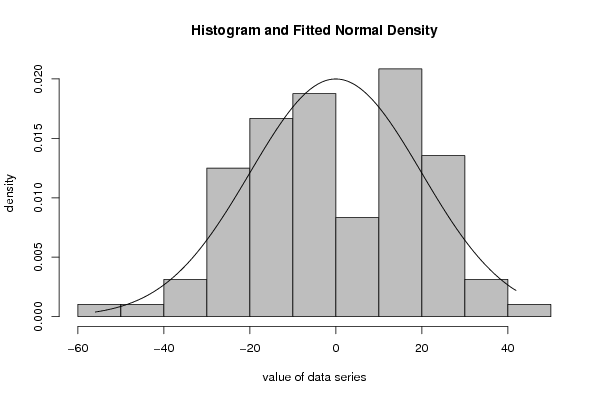
Title produced by software

Maximum-likelihood Fitting - Normal Distribution

Date of computation

Tue, 16 Dec 2008 13:13:47 -0700

Cite this page as follows

Statistical Computations at FreeStatistics.org, Office for Research Development and Education, URL https://freestatistics.org/blog/index.php?v=date/2008/Dec/16/t1229458487fiv7gf5n7dv7avi.htm/, Retrieved Wed, 15 May 2024 13:53:14 +0000

Statistical Computations at FreeStatistics.org, Office for Research Development and Education, URL https://freestatistics.org/blog/index.php?pk=34168, Retrieved Wed, 15 May 2024 13:53:14 +0000

QR Codes:

Paste this QR Code to cite your computation.

Original text written by user:

IsPrivate?

No (this computation is public)

User-defined keywords

Estimated Impact

226

Family? (F = Feedback message, R = changed R code, M = changed R Module, P = changed Parameters, D = changed Data)

-     [Central Tendency] [Central tendency ...] [2008-12-07 15:13:41] [c45c87b96bbf32ffc2144fc37d767b2e]
- RMPD  [Maximum-likelihood Fitting - Normal Distribution] [distribution] [2008-12-14 15:37:18] [c45c87b96bbf32ffc2144fc37d767b2e]
-    D      [Maximum-likelihood Fitting - Normal Distribution] [distribution] [2008-12-16 20:13:47] [3dc594a6c62226e1e98766c4d385bfaa] [Current]
-  MPD        [Maximum-likelihood Fitting - Normal Distribution] [] [2009-12-30 20:05:53] [d2d412c7f4d35ffbf5ee5ee89db327d4] 

Feedback Forum

Post a new message

Dataseries X:

Download CSV

Histogram

Boxplots

24.70833333
35.58333333
21.33333333
14.58333333
15.08333333
14.95833333
13.08333333
6.083333333
-2.791666667
-1.041666667
-7.916666667
-10.29166667
-16.5625
-0.6875
-14.9375
-16.6875
-18.1875
-22.3125
-18.1875
-20.1875
-22.0625
-20.3125
-19.1875
-23.5625
-25.83333333
-16.95833333
-8.208333333
-3.958333333
-16.45833333
-16.58333333
-14.45833333
-10.45833333
-5.333333333
-7.583333333
-5.458333333
-3.833333333
1.895833333
-7.229166667
-3.479166667
6.770833333
16.27083333
19.14583333
23.27083333
26.27083333
29.39583333
35.14583333
35.27083333
41.89583333
-20.14583333
-26.27083333
-22.52083333
-21.27083333
-19.77083333
-11.89583333
-7.770833333
-3.770833333
0.354166667
-3.895833333
-2.770833333
3.854166667
-0.416666667
-0.541666667
7.208333333
19.45833333
21.95833333
22.83333333
15.95833333
18.95833333
24.08333333
19.83333333
21.95833333
24.58333333
21.3125
12.1875
16.9375
15.1875
17.6875
19.5625
12.6875
14.6875
14.8125
15.5625
22.6875
23.3125
15.04166667
3.916666667
3.666666667
-14.08333333
-16.58333333
-25.70833333
-24.58333333
-31.58333333
-38.45833333
-37.70833333
-44.58333333
-55.95833333

Summary of computational transaction
Raw Input	view raw input (R code)
Raw Output	view raw output of R engine
Computing time	2 seconds
R Server	'Herman Ole Andreas Wold' @ 193.190.124.10:1001

\begin{tabular}{lllllllll}
\hline
Summary of computational transaction \tabularnewline
Raw Input & view raw input (R code)  \tabularnewline
Raw Output & view raw output of R engine  \tabularnewline
Computing time & 2 seconds \tabularnewline
R Server & 'Herman Ole Andreas Wold' @ 193.190.124.10:1001 \tabularnewline
\hline
\end{tabular}
%Source: https://freestatistics.org/blog/index.php?pk=34168&T=0

[TABLE]
[ROW][C]Summary of computational transaction[/C][/ROW]
[ROW][C]Raw Input[/C][C]view raw input (R code) [/C][/ROW]
[ROW][C]Raw Output[/C][C]view raw output of R engine [/C][/ROW]
[ROW][C]Computing time[/C][C]2 seconds[/C][/ROW]
[ROW][C]R Server[/C][C]'Herman Ole Andreas Wold' @ 193.190.124.10:1001[/C][/ROW]
[/TABLE]
Source: https://freestatistics.org/blog/index.php?pk=34168&T=0

Globally Unique Identifier (entire table): ba.freestatistics.org/blog/index.php?pk=34168&T=0

As an alternative you can also use a QR Code:

The GUIDs for individual cells are displayed in the table below:

Summary of computational transaction
Raw Input	view raw input (R code)
Raw Output	view raw output of R engine
Computing time	2 seconds
R Server	'Herman Ole Andreas Wold' @ 193.190.124.10:1001

Parameter	Estimated Value	Standard Deviation
mean	-9.37500441138226e-11	2.03560064240797
standard deviation	19.9447315759247	1.43938701803437

\begin{tabular}{lllllllll}
\hline
Parameter & Estimated Value & Standard Deviation \tabularnewline
mean & -9.37500441138226e-11 & 2.03560064240797 \tabularnewline
standard deviation & 19.9447315759247 & 1.43938701803437 \tabularnewline
\hline
\end{tabular}
%Source: https://freestatistics.org/blog/index.php?pk=34168&T=1

[TABLE]
[ROW][C]Parameter[/C][C]Estimated Value[/C][C]Standard Deviation[/C][/ROW]
[ROW][C]mean[/C][C]-9.37500441138226e-11[/C][C]2.03560064240797[/C][/ROW]
[ROW][C]standard deviation[/C][C]19.9447315759247[/C][C]1.43938701803437[/C][/ROW]
[/TABLE]
Source: https://freestatistics.org/blog/index.php?pk=34168&T=1

Globally Unique Identifier (entire table): ba.freestatistics.org/blog/index.php?pk=34168&T=1

As an alternative you can also use a QR Code:

The GUIDs for individual cells are displayed in the table below:

Parameter	Estimated Value	Standard Deviation
mean	-9.37500441138226e-11	2.03560064240797
standard deviation	19.9447315759247	1.43938701803437

Figure 1

PNG link

Postscript link

PDF link

Parameters (Session):

par1 = 8 ; par2 = 0 ;

Parameters (R input):

par1 = 8 ; par2 = 0 ;

R code (references can be found in the software module):

library(MASS)
par1 <- as.numeric(par1)
if (par2 == '0') par2 = 'Sturges' else par2 <- as.numeric(par2)
x <- as.ts(x) #otherwise the fitdistr function does not work properly
r <- fitdistr(x,'normal')
r
bitmap(file='test1.png')
myhist<-hist(x,col=par1,breaks=par2,main=main,ylab=ylab,xlab=xlab,freq=F)
curve(1/(r$estimate[2]*sqrt(2*pi))*exp(-1/2*((x-r$estimate[1])/r$estimate[2])^2),min(x),max(x),add=T)
dev.off()
load(file='createtable')
a<-table.start()
a<-table.row.start(a)
a<-table.element(a,'Parameter',1,TRUE)
a<-table.element(a,'Estimated Value',1,TRUE)
a<-table.element(a,'Standard Deviation',1,TRUE)
a<-table.row.end(a)
a<-table.row.start(a)
a<-table.element(a,'mean',header=TRUE)
a<-table.element(a,r$estimate[1])
a<-table.element(a,r$sd[1])
a<-table.row.end(a)
a<-table.row.start(a)
a<-table.element(a,'standard deviation',header=TRUE)
a<-table.element(a,r$estimate[2])
a<-table.element(a,r$sd[2])
a<-table.row.end(a)
a<-table.end(a)
table.save(a,file='mytable.tab')

Free Statistics

Description of Statistical Computation

Tree of Dependent Computations

Dataset

Tables (Output of Computation)

Figures (Output of Computation)

Input Parameters & R Code