Repository of Reproducible Computations

Free Statistics

of Irreproducible Research!

Author's title

Author

*The author of this computation has been verified*

R Software Module

rwasp_autocorrelation.wasp

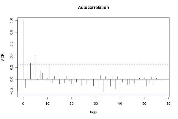
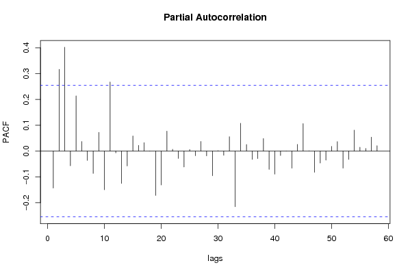
Title produced by software

(Partial) Autocorrelation Function

Date of computation

Tue, 16 Dec 2008 11:12:47 -0700

Cite this page as follows

Statistical Computations at FreeStatistics.org, Office for Research Development and Education, URL https://freestatistics.org/blog/index.php?v=date/2008/Dec/16/t12294512951lclke46d6t175i.htm/, Retrieved Wed, 15 May 2024 21:43:15 +0000

Statistical Computations at FreeStatistics.org, Office for Research Development and Education, URL https://freestatistics.org/blog/index.php?pk=34077, Retrieved Wed, 15 May 2024 21:43:15 +0000

QR Codes:

Paste this QR Code to cite your computation.

Original text written by user:

IsPrivate?

No (this computation is public)

User-defined keywords

Estimated Impact

169

Family? (F = Feedback message, R = changed R code, M = changed R Module, P = changed Parameters, D = changed Data)

-     [(Partial) Autocorrelation Function] [ACF na transformatie] [2008-12-10 16:07:27] [2a0ad3a9bcadca2da0acb91636601c6c]
-    D  [(Partial) Autocorrelation Function] [AutoCorrelation F...] [2008-12-11 17:57:12] [888addc516c3b812dd7be4bd54caa358]
-           [(Partial) Autocorrelation Function] [] [2008-12-16 18:12:47] [4f54996111e63ee83b19b6a8540c6bad] [Current]

Feedback Forum

Post a new message

Dataseries X:

Download CSV

Histogram

Boxplots

5,7
5,7
5,6
5,8
5,6
5,6
5,6
5,5
5,4
5,4
5,5
5,4
5,4
5,2
5,4
5,2
5,1
5,1
5,0
5,0
4,9
5,1
5,0
5,0
4,8
4,7
4,7
4,7
4,7
4,7
4,6
4,7
4,7
4,5
4,4
4,5
4,4
4,6
4,5
4,4
4,5
4,5
4,6
4,7
4,7
4,7
4,8
4,7
5,0
4,9
4,8
5,1
5,0
5,5
5,5
5,7
6,1
6,1
6,5
6,7

Summary of computational transaction
Raw Input	view raw input (R code)
Raw Output	view raw output of R engine
Computing time	2 seconds
R Server	'Sir Ronald Aylmer Fisher' @ 193.190.124.24

\begin{tabular}{lllllllll}
\hline
Summary of computational transaction \tabularnewline
Raw Input & view raw input (R code)  \tabularnewline
Raw Output & view raw output of R engine  \tabularnewline
Computing time & 2 seconds \tabularnewline
R Server & 'Sir Ronald Aylmer Fisher' @ 193.190.124.24 \tabularnewline
\hline
\end{tabular}
%Source: https://freestatistics.org/blog/index.php?pk=34077&T=0

[TABLE]
[ROW][C]Summary of computational transaction[/C][/ROW]
[ROW][C]Raw Input[/C][C]view raw input (R code) [/C][/ROW]
[ROW][C]Raw Output[/C][C]view raw output of R engine [/C][/ROW]
[ROW][C]Computing time[/C][C]2 seconds[/C][/ROW]
[ROW][C]R Server[/C][C]'Sir Ronald Aylmer Fisher' @ 193.190.124.24[/C][/ROW]
[/TABLE]
Source: https://freestatistics.org/blog/index.php?pk=34077&T=0

Globally Unique Identifier (entire table): ba.freestatistics.org/blog/index.php?pk=34077&T=0

As an alternative you can also use a QR Code:

The GUIDs for individual cells are displayed in the table below:

Summary of computational transaction
Raw Input	view raw input (R code)
Raw Output	view raw output of R engine
Computing time	2 seconds
R Server	'Sir Ronald Aylmer Fisher' @ 193.190.124.24

Autocorrelation Function
Time lag k	ACF(k)	T-STAT	P-value
1	-0.143246	-1.1003	0.137836
2	0.330945	2.542	0.006834
3	0.276907	2.127	0.018807
4	-0.044161	-0.3392	0.367828
5	0.407757	3.132	0.001351
6	-0.014074	-0.1081	0.457138
7	0.145085	1.1144	0.134809
8	0.107365	0.8247	0.206435
9	0.061547	0.4727	0.319068
10	0.012155	0.0934	0.462966
11	0.262548	2.0167	0.024144
12	-0.064357	-0.4943	0.311453
13	0.05133	0.3943	0.347401
14	0.103891	0.798	0.214034
15	-0.081399	-0.6252	0.267114
16	0.205322	1.5771	0.060059
17	-0.060721	-0.4664	0.321321
18	0.051512	0.3957	0.346888
19	-0.040043	-0.3076	0.379743
20	-0.075381	-0.579	0.282393
21	0.059124	0.4541	0.325697
22	-0.048867	-0.3754	0.354371
23	-0.025605	-0.1967	0.422377
24	-0.106679	-0.8194	0.207923
25	-0.008501	-0.0653	0.47408
26	-0.073138	-0.5618	0.288195
27	0.001577	0.0121	0.495189
28	-0.054842	-0.4213	0.33755
29	-0.110071	-0.8455	0.200633
30	-0.021302	-0.1636	0.435295
31	-0.139774	-1.0736	0.143681
32	0.063812	0.4901	0.312924
33	-0.219859	-1.6888	0.048272
34	0.04578	0.3516	0.363178
35	-0.1301	-0.9993	0.160861
36	-0.119821	-0.9204	0.180566
37	0.043984	0.3378	0.368339
38	-0.169415	-1.3013	0.099107
39	0.042389	0.3256	0.372941
40	-0.203763	-1.5651	0.06145
41	-0.049368	-0.3792	0.35295
42	-0.056597	-0.4347	0.332673
43	-0.090743	-0.697	0.244266
44	-0.078082	-0.5998	0.275482
45	-0.024449	-0.1878	0.425841
46	-0.070268	-0.5397	0.295706
47	-0.109178	-0.8386	0.202535
48	0.020682	0.1589	0.437161
49	-0.1365	-1.0485	0.149348
50	0.03195	0.2454	0.403494
51	-0.119276	-0.9162	0.181652
52	-0.058615	-0.4502	0.327096
53	0.030273	0.2325	0.408466
54	-0.096418	-0.7406	0.230936
55	0.018197	0.1398	0.444658
56	-0.007732	-0.0594	0.476422
57	-0.019606	-0.1506	0.440404
58	-0.00218	-0.0167	0.493348
59	NA	NA	NA
60	NA	NA	NA

\begin{tabular}{lllllllll}
\hline
Autocorrelation Function \tabularnewline
Time lag k & ACF(k) & T-STAT & P-value \tabularnewline
1 & -0.143246 & -1.1003 & 0.137836 \tabularnewline
2 & 0.330945 & 2.542 & 0.006834 \tabularnewline
3 & 0.276907 & 2.127 & 0.018807 \tabularnewline
4 & -0.044161 & -0.3392 & 0.367828 \tabularnewline
5 & 0.407757 & 3.132 & 0.001351 \tabularnewline
6 & -0.014074 & -0.1081 & 0.457138 \tabularnewline
7 & 0.145085 & 1.1144 & 0.134809 \tabularnewline
8 & 0.107365 & 0.8247 & 0.206435 \tabularnewline
9 & 0.061547 & 0.4727 & 0.319068 \tabularnewline
10 & 0.012155 & 0.0934 & 0.462966 \tabularnewline
11 & 0.262548 & 2.0167 & 0.024144 \tabularnewline
12 & -0.064357 & -0.4943 & 0.311453 \tabularnewline
13 & 0.05133 & 0.3943 & 0.347401 \tabularnewline
14 & 0.103891 & 0.798 & 0.214034 \tabularnewline
15 & -0.081399 & -0.6252 & 0.267114 \tabularnewline
16 & 0.205322 & 1.5771 & 0.060059 \tabularnewline
17 & -0.060721 & -0.4664 & 0.321321 \tabularnewline
18 & 0.051512 & 0.3957 & 0.346888 \tabularnewline
19 & -0.040043 & -0.3076 & 0.379743 \tabularnewline
20 & -0.075381 & -0.579 & 0.282393 \tabularnewline
21 & 0.059124 & 0.4541 & 0.325697 \tabularnewline
22 & -0.048867 & -0.3754 & 0.354371 \tabularnewline
23 & -0.025605 & -0.1967 & 0.422377 \tabularnewline
24 & -0.106679 & -0.8194 & 0.207923 \tabularnewline
25 & -0.008501 & -0.0653 & 0.47408 \tabularnewline
26 & -0.073138 & -0.5618 & 0.288195 \tabularnewline
27 & 0.001577 & 0.0121 & 0.495189 \tabularnewline
28 & -0.054842 & -0.4213 & 0.33755 \tabularnewline
29 & -0.110071 & -0.8455 & 0.200633 \tabularnewline
30 & -0.021302 & -0.1636 & 0.435295 \tabularnewline
31 & -0.139774 & -1.0736 & 0.143681 \tabularnewline
32 & 0.063812 & 0.4901 & 0.312924 \tabularnewline
33 & -0.219859 & -1.6888 & 0.048272 \tabularnewline
34 & 0.04578 & 0.3516 & 0.363178 \tabularnewline
35 & -0.1301 & -0.9993 & 0.160861 \tabularnewline
36 & -0.119821 & -0.9204 & 0.180566 \tabularnewline
37 & 0.043984 & 0.3378 & 0.368339 \tabularnewline
38 & -0.169415 & -1.3013 & 0.099107 \tabularnewline
39 & 0.042389 & 0.3256 & 0.372941 \tabularnewline
40 & -0.203763 & -1.5651 & 0.06145 \tabularnewline
41 & -0.049368 & -0.3792 & 0.35295 \tabularnewline
42 & -0.056597 & -0.4347 & 0.332673 \tabularnewline
43 & -0.090743 & -0.697 & 0.244266 \tabularnewline
44 & -0.078082 & -0.5998 & 0.275482 \tabularnewline
45 & -0.024449 & -0.1878 & 0.425841 \tabularnewline
46 & -0.070268 & -0.5397 & 0.295706 \tabularnewline
47 & -0.109178 & -0.8386 & 0.202535 \tabularnewline
48 & 0.020682 & 0.1589 & 0.437161 \tabularnewline
49 & -0.1365 & -1.0485 & 0.149348 \tabularnewline
50 & 0.03195 & 0.2454 & 0.403494 \tabularnewline
51 & -0.119276 & -0.9162 & 0.181652 \tabularnewline
52 & -0.058615 & -0.4502 & 0.327096 \tabularnewline
53 & 0.030273 & 0.2325 & 0.408466 \tabularnewline
54 & -0.096418 & -0.7406 & 0.230936 \tabularnewline
55 & 0.018197 & 0.1398 & 0.444658 \tabularnewline
56 & -0.007732 & -0.0594 & 0.476422 \tabularnewline
57 & -0.019606 & -0.1506 & 0.440404 \tabularnewline
58 & -0.00218 & -0.0167 & 0.493348 \tabularnewline
59 & NA & NA & NA \tabularnewline
60 & NA & NA & NA \tabularnewline
\hline
\end{tabular}
%Source: https://freestatistics.org/blog/index.php?pk=34077&T=1

[TABLE]
[ROW][C]Autocorrelation Function[/C][/ROW]
[ROW][C]Time lag k[/C][C]ACF(k)[/C][C]T-STAT[/C][C]P-value[/C][/ROW]
[ROW][C]1[/C][C]-0.143246[/C][C]-1.1003[/C][C]0.137836[/C][/ROW]
[ROW][C]2[/C][C]0.330945[/C][C]2.542[/C][C]0.006834[/C][/ROW]
[ROW][C]3[/C][C]0.276907[/C][C]2.127[/C][C]0.018807[/C][/ROW]
[ROW][C]4[/C][C]-0.044161[/C][C]-0.3392[/C][C]0.367828[/C][/ROW]
[ROW][C]5[/C][C]0.407757[/C][C]3.132[/C][C]0.001351[/C][/ROW]
[ROW][C]6[/C][C]-0.014074[/C][C]-0.1081[/C][C]0.457138[/C][/ROW]
[ROW][C]7[/C][C]0.145085[/C][C]1.1144[/C][C]0.134809[/C][/ROW]
[ROW][C]8[/C][C]0.107365[/C][C]0.8247[/C][C]0.206435[/C][/ROW]
[ROW][C]9[/C][C]0.061547[/C][C]0.4727[/C][C]0.319068[/C][/ROW]
[ROW][C]10[/C][C]0.012155[/C][C]0.0934[/C][C]0.462966[/C][/ROW]
[ROW][C]11[/C][C]0.262548[/C][C]2.0167[/C][C]0.024144[/C][/ROW]
[ROW][C]12[/C][C]-0.064357[/C][C]-0.4943[/C][C]0.311453[/C][/ROW]
[ROW][C]13[/C][C]0.05133[/C][C]0.3943[/C][C]0.347401[/C][/ROW]
[ROW][C]14[/C][C]0.103891[/C][C]0.798[/C][C]0.214034[/C][/ROW]
[ROW][C]15[/C][C]-0.081399[/C][C]-0.6252[/C][C]0.267114[/C][/ROW]
[ROW][C]16[/C][C]0.205322[/C][C]1.5771[/C][C]0.060059[/C][/ROW]
[ROW][C]17[/C][C]-0.060721[/C][C]-0.4664[/C][C]0.321321[/C][/ROW]
[ROW][C]18[/C][C]0.051512[/C][C]0.3957[/C][C]0.346888[/C][/ROW]
[ROW][C]19[/C][C]-0.040043[/C][C]-0.3076[/C][C]0.379743[/C][/ROW]
[ROW][C]20[/C][C]-0.075381[/C][C]-0.579[/C][C]0.282393[/C][/ROW]
[ROW][C]21[/C][C]0.059124[/C][C]0.4541[/C][C]0.325697[/C][/ROW]
[ROW][C]22[/C][C]-0.048867[/C][C]-0.3754[/C][C]0.354371[/C][/ROW]
[ROW][C]23[/C][C]-0.025605[/C][C]-0.1967[/C][C]0.422377[/C][/ROW]
[ROW][C]24[/C][C]-0.106679[/C][C]-0.8194[/C][C]0.207923[/C][/ROW]
[ROW][C]25[/C][C]-0.008501[/C][C]-0.0653[/C][C]0.47408[/C][/ROW]
[ROW][C]26[/C][C]-0.073138[/C][C]-0.5618[/C][C]0.288195[/C][/ROW]
[ROW][C]27[/C][C]0.001577[/C][C]0.0121[/C][C]0.495189[/C][/ROW]
[ROW][C]28[/C][C]-0.054842[/C][C]-0.4213[/C][C]0.33755[/C][/ROW]
[ROW][C]29[/C][C]-0.110071[/C][C]-0.8455[/C][C]0.200633[/C][/ROW]
[ROW][C]30[/C][C]-0.021302[/C][C]-0.1636[/C][C]0.435295[/C][/ROW]
[ROW][C]31[/C][C]-0.139774[/C][C]-1.0736[/C][C]0.143681[/C][/ROW]
[ROW][C]32[/C][C]0.063812[/C][C]0.4901[/C][C]0.312924[/C][/ROW]
[ROW][C]33[/C][C]-0.219859[/C][C]-1.6888[/C][C]0.048272[/C][/ROW]
[ROW][C]34[/C][C]0.04578[/C][C]0.3516[/C][C]0.363178[/C][/ROW]
[ROW][C]35[/C][C]-0.1301[/C][C]-0.9993[/C][C]0.160861[/C][/ROW]
[ROW][C]36[/C][C]-0.119821[/C][C]-0.9204[/C][C]0.180566[/C][/ROW]
[ROW][C]37[/C][C]0.043984[/C][C]0.3378[/C][C]0.368339[/C][/ROW]
[ROW][C]38[/C][C]-0.169415[/C][C]-1.3013[/C][C]0.099107[/C][/ROW]
[ROW][C]39[/C][C]0.042389[/C][C]0.3256[/C][C]0.372941[/C][/ROW]
[ROW][C]40[/C][C]-0.203763[/C][C]-1.5651[/C][C]0.06145[/C][/ROW]
[ROW][C]41[/C][C]-0.049368[/C][C]-0.3792[/C][C]0.35295[/C][/ROW]
[ROW][C]42[/C][C]-0.056597[/C][C]-0.4347[/C][C]0.332673[/C][/ROW]
[ROW][C]43[/C][C]-0.090743[/C][C]-0.697[/C][C]0.244266[/C][/ROW]
[ROW][C]44[/C][C]-0.078082[/C][C]-0.5998[/C][C]0.275482[/C][/ROW]
[ROW][C]45[/C][C]-0.024449[/C][C]-0.1878[/C][C]0.425841[/C][/ROW]
[ROW][C]46[/C][C]-0.070268[/C][C]-0.5397[/C][C]0.295706[/C][/ROW]
[ROW][C]47[/C][C]-0.109178[/C][C]-0.8386[/C][C]0.202535[/C][/ROW]
[ROW][C]48[/C][C]0.020682[/C][C]0.1589[/C][C]0.437161[/C][/ROW]
[ROW][C]49[/C][C]-0.1365[/C][C]-1.0485[/C][C]0.149348[/C][/ROW]
[ROW][C]50[/C][C]0.03195[/C][C]0.2454[/C][C]0.403494[/C][/ROW]
[ROW][C]51[/C][C]-0.119276[/C][C]-0.9162[/C][C]0.181652[/C][/ROW]
[ROW][C]52[/C][C]-0.058615[/C][C]-0.4502[/C][C]0.327096[/C][/ROW]
[ROW][C]53[/C][C]0.030273[/C][C]0.2325[/C][C]0.408466[/C][/ROW]
[ROW][C]54[/C][C]-0.096418[/C][C]-0.7406[/C][C]0.230936[/C][/ROW]
[ROW][C]55[/C][C]0.018197[/C][C]0.1398[/C][C]0.444658[/C][/ROW]
[ROW][C]56[/C][C]-0.007732[/C][C]-0.0594[/C][C]0.476422[/C][/ROW]
[ROW][C]57[/C][C]-0.019606[/C][C]-0.1506[/C][C]0.440404[/C][/ROW]
[ROW][C]58[/C][C]-0.00218[/C][C]-0.0167[/C][C]0.493348[/C][/ROW]
[ROW][C]59[/C][C]NA[/C][C]NA[/C][C]NA[/C][/ROW]
[ROW][C]60[/C][C]NA[/C][C]NA[/C][C]NA[/C][/ROW]
[/TABLE]
Source: https://freestatistics.org/blog/index.php?pk=34077&T=1

Globally Unique Identifier (entire table): ba.freestatistics.org/blog/index.php?pk=34077&T=1

As an alternative you can also use a QR Code:

The GUIDs for individual cells are displayed in the table below:

Autocorrelation Function
Time lag k	ACF(k)	T-STAT	P-value
1	-0.143246	-1.1003	0.137836
2	0.330945	2.542	0.006834
3	0.276907	2.127	0.018807
4	-0.044161	-0.3392	0.367828
5	0.407757	3.132	0.001351
6	-0.014074	-0.1081	0.457138
7	0.145085	1.1144	0.134809
8	0.107365	0.8247	0.206435
9	0.061547	0.4727	0.319068
10	0.012155	0.0934	0.462966
11	0.262548	2.0167	0.024144
12	-0.064357	-0.4943	0.311453
13	0.05133	0.3943	0.347401
14	0.103891	0.798	0.214034
15	-0.081399	-0.6252	0.267114
16	0.205322	1.5771	0.060059
17	-0.060721	-0.4664	0.321321
18	0.051512	0.3957	0.346888
19	-0.040043	-0.3076	0.379743
20	-0.075381	-0.579	0.282393
21	0.059124	0.4541	0.325697
22	-0.048867	-0.3754	0.354371
23	-0.025605	-0.1967	0.422377
24	-0.106679	-0.8194	0.207923
25	-0.008501	-0.0653	0.47408
26	-0.073138	-0.5618	0.288195
27	0.001577	0.0121	0.495189
28	-0.054842	-0.4213	0.33755
29	-0.110071	-0.8455	0.200633
30	-0.021302	-0.1636	0.435295
31	-0.139774	-1.0736	0.143681
32	0.063812	0.4901	0.312924
33	-0.219859	-1.6888	0.048272
34	0.04578	0.3516	0.363178
35	-0.1301	-0.9993	0.160861
36	-0.119821	-0.9204	0.180566
37	0.043984	0.3378	0.368339
38	-0.169415	-1.3013	0.099107
39	0.042389	0.3256	0.372941
40	-0.203763	-1.5651	0.06145
41	-0.049368	-0.3792	0.35295
42	-0.056597	-0.4347	0.332673
43	-0.090743	-0.697	0.244266
44	-0.078082	-0.5998	0.275482
45	-0.024449	-0.1878	0.425841
46	-0.070268	-0.5397	0.295706
47	-0.109178	-0.8386	0.202535
48	0.020682	0.1589	0.437161
49	-0.1365	-1.0485	0.149348
50	0.03195	0.2454	0.403494
51	-0.119276	-0.9162	0.181652
52	-0.058615	-0.4502	0.327096
53	0.030273	0.2325	0.408466
54	-0.096418	-0.7406	0.230936
55	0.018197	0.1398	0.444658
56	-0.007732	-0.0594	0.476422
57	-0.019606	-0.1506	0.440404
58	-0.00218	-0.0167	0.493348
59	NA	NA	NA
60	NA	NA	NA

Partial Autocorrelation Function
Time lag k	PACF(k)	T-STAT	P-value
1	-0.143246	-1.1003	0.137836
2	0.316928	2.4344	0.008981
3	0.402553	3.0921	0.001517
4	-0.056881	-0.4369	0.331887
5	0.213888	1.6429	0.052861
6	0.037036	0.2845	0.38852
7	-0.036187	-0.278	0.39101
8	-0.086592	-0.6651	0.254281
9	0.072589	0.5576	0.289626
10	-0.14989	-1.1513	0.127122
11	0.267847	2.0574	0.022039
12	-0.006851	-0.0526	0.479104
13	-0.12535	-0.9628	0.16978
14	-0.057473	-0.4415	0.330247
15	0.058794	0.4516	0.326605
16	0.021915	0.1683	0.433449
17	0.032815	0.2521	0.400936
18	-0.000439	-0.0034	0.498661
19	-0.171628	-1.3183	0.096249
20	-0.131391	-1.0092	0.158492
21	0.077288	0.5937	0.277504
22	0.007063	0.0543	0.478457
23	-0.028524	-0.2191	0.413665
24	-0.061515	-0.4725	0.319154
25	0.005899	0.0453	0.482006
26	-0.01798	-0.1381	0.445312
27	0.037331	0.2867	0.387655
28	-0.018335	-0.1408	0.44424
29	-0.095322	-0.7322	0.233477
30	0.001387	0.0107	0.495767
31	-0.016232	-0.1247	0.450602
32	0.055624	0.4273	0.335374
33	-0.215674	-1.6566	0.051453
34	0.107877	0.8286	0.205331
35	0.025433	0.1954	0.422894
36	-0.032121	-0.2467	0.402987
37	-0.029315	-0.2252	0.411312
38	0.048719	0.3742	0.354792
39	-0.071124	-0.5463	0.293455
40	-0.089293	-0.6859	0.24774
41	-0.017354	-0.1333	0.447205
42	-0.000157	-0.0012	0.499522
43	-0.066313	-0.5094	0.3062
44	0.025856	0.1986	0.421626
45	0.106311	0.8166	0.208723
46	0.00046	0.0035	0.498597
47	-0.082215	-0.6315	0.265075
48	-0.046369	-0.3562	0.361492
49	-0.034883	-0.2679	0.394839
50	0.018155	0.1394	0.444785
51	0.036724	0.2821	0.389434
52	-0.066045	-0.5073	0.306918
53	-0.032171	-0.2471	0.402841
54	0.081053	0.6226	0.267979
55	0.014755	0.1133	0.455075
56	0.009932	0.0763	0.469725
57	0.054109	0.4156	0.339598
58	0.020607	0.1583	0.437385
59	NA	NA	NA
60	NA	NA	NA

\begin{tabular}{lllllllll}
\hline
Partial Autocorrelation Function \tabularnewline
Time lag k & PACF(k) & T-STAT & P-value \tabularnewline
1 & -0.143246 & -1.1003 & 0.137836 \tabularnewline
2 & 0.316928 & 2.4344 & 0.008981 \tabularnewline
3 & 0.402553 & 3.0921 & 0.001517 \tabularnewline
4 & -0.056881 & -0.4369 & 0.331887 \tabularnewline
5 & 0.213888 & 1.6429 & 0.052861 \tabularnewline
6 & 0.037036 & 0.2845 & 0.38852 \tabularnewline
7 & -0.036187 & -0.278 & 0.39101 \tabularnewline
8 & -0.086592 & -0.6651 & 0.254281 \tabularnewline
9 & 0.072589 & 0.5576 & 0.289626 \tabularnewline
10 & -0.14989 & -1.1513 & 0.127122 \tabularnewline
11 & 0.267847 & 2.0574 & 0.022039 \tabularnewline
12 & -0.006851 & -0.0526 & 0.479104 \tabularnewline
13 & -0.12535 & -0.9628 & 0.16978 \tabularnewline
14 & -0.057473 & -0.4415 & 0.330247 \tabularnewline
15 & 0.058794 & 0.4516 & 0.326605 \tabularnewline
16 & 0.021915 & 0.1683 & 0.433449 \tabularnewline
17 & 0.032815 & 0.2521 & 0.400936 \tabularnewline
18 & -0.000439 & -0.0034 & 0.498661 \tabularnewline
19 & -0.171628 & -1.3183 & 0.096249 \tabularnewline
20 & -0.131391 & -1.0092 & 0.158492 \tabularnewline
21 & 0.077288 & 0.5937 & 0.277504 \tabularnewline
22 & 0.007063 & 0.0543 & 0.478457 \tabularnewline
23 & -0.028524 & -0.2191 & 0.413665 \tabularnewline
24 & -0.061515 & -0.4725 & 0.319154 \tabularnewline
25 & 0.005899 & 0.0453 & 0.482006 \tabularnewline
26 & -0.01798 & -0.1381 & 0.445312 \tabularnewline
27 & 0.037331 & 0.2867 & 0.387655 \tabularnewline
28 & -0.018335 & -0.1408 & 0.44424 \tabularnewline
29 & -0.095322 & -0.7322 & 0.233477 \tabularnewline
30 & 0.001387 & 0.0107 & 0.495767 \tabularnewline
31 & -0.016232 & -0.1247 & 0.450602 \tabularnewline
32 & 0.055624 & 0.4273 & 0.335374 \tabularnewline
33 & -0.215674 & -1.6566 & 0.051453 \tabularnewline
34 & 0.107877 & 0.8286 & 0.205331 \tabularnewline
35 & 0.025433 & 0.1954 & 0.422894 \tabularnewline
36 & -0.032121 & -0.2467 & 0.402987 \tabularnewline
37 & -0.029315 & -0.2252 & 0.411312 \tabularnewline
38 & 0.048719 & 0.3742 & 0.354792 \tabularnewline
39 & -0.071124 & -0.5463 & 0.293455 \tabularnewline
40 & -0.089293 & -0.6859 & 0.24774 \tabularnewline
41 & -0.017354 & -0.1333 & 0.447205 \tabularnewline
42 & -0.000157 & -0.0012 & 0.499522 \tabularnewline
43 & -0.066313 & -0.5094 & 0.3062 \tabularnewline
44 & 0.025856 & 0.1986 & 0.421626 \tabularnewline
45 & 0.106311 & 0.8166 & 0.208723 \tabularnewline
46 & 0.00046 & 0.0035 & 0.498597 \tabularnewline
47 & -0.082215 & -0.6315 & 0.265075 \tabularnewline
48 & -0.046369 & -0.3562 & 0.361492 \tabularnewline
49 & -0.034883 & -0.2679 & 0.394839 \tabularnewline
50 & 0.018155 & 0.1394 & 0.444785 \tabularnewline
51 & 0.036724 & 0.2821 & 0.389434 \tabularnewline
52 & -0.066045 & -0.5073 & 0.306918 \tabularnewline
53 & -0.032171 & -0.2471 & 0.402841 \tabularnewline
54 & 0.081053 & 0.6226 & 0.267979 \tabularnewline
55 & 0.014755 & 0.1133 & 0.455075 \tabularnewline
56 & 0.009932 & 0.0763 & 0.469725 \tabularnewline
57 & 0.054109 & 0.4156 & 0.339598 \tabularnewline
58 & 0.020607 & 0.1583 & 0.437385 \tabularnewline
59 & NA & NA & NA \tabularnewline
60 & NA & NA & NA \tabularnewline
\hline
\end{tabular}
%Source: https://freestatistics.org/blog/index.php?pk=34077&T=2

[TABLE]
[ROW][C]Partial Autocorrelation Function[/C][/ROW]
[ROW][C]Time lag k[/C][C]PACF(k)[/C][C]T-STAT[/C][C]P-value[/C][/ROW]
[ROW][C]1[/C][C]-0.143246[/C][C]-1.1003[/C][C]0.137836[/C][/ROW]
[ROW][C]2[/C][C]0.316928[/C][C]2.4344[/C][C]0.008981[/C][/ROW]
[ROW][C]3[/C][C]0.402553[/C][C]3.0921[/C][C]0.001517[/C][/ROW]
[ROW][C]4[/C][C]-0.056881[/C][C]-0.4369[/C][C]0.331887[/C][/ROW]
[ROW][C]5[/C][C]0.213888[/C][C]1.6429[/C][C]0.052861[/C][/ROW]
[ROW][C]6[/C][C]0.037036[/C][C]0.2845[/C][C]0.38852[/C][/ROW]
[ROW][C]7[/C][C]-0.036187[/C][C]-0.278[/C][C]0.39101[/C][/ROW]
[ROW][C]8[/C][C]-0.086592[/C][C]-0.6651[/C][C]0.254281[/C][/ROW]
[ROW][C]9[/C][C]0.072589[/C][C]0.5576[/C][C]0.289626[/C][/ROW]
[ROW][C]10[/C][C]-0.14989[/C][C]-1.1513[/C][C]0.127122[/C][/ROW]
[ROW][C]11[/C][C]0.267847[/C][C]2.0574[/C][C]0.022039[/C][/ROW]
[ROW][C]12[/C][C]-0.006851[/C][C]-0.0526[/C][C]0.479104[/C][/ROW]
[ROW][C]13[/C][C]-0.12535[/C][C]-0.9628[/C][C]0.16978[/C][/ROW]
[ROW][C]14[/C][C]-0.057473[/C][C]-0.4415[/C][C]0.330247[/C][/ROW]
[ROW][C]15[/C][C]0.058794[/C][C]0.4516[/C][C]0.326605[/C][/ROW]
[ROW][C]16[/C][C]0.021915[/C][C]0.1683[/C][C]0.433449[/C][/ROW]
[ROW][C]17[/C][C]0.032815[/C][C]0.2521[/C][C]0.400936[/C][/ROW]
[ROW][C]18[/C][C]-0.000439[/C][C]-0.0034[/C][C]0.498661[/C][/ROW]
[ROW][C]19[/C][C]-0.171628[/C][C]-1.3183[/C][C]0.096249[/C][/ROW]
[ROW][C]20[/C][C]-0.131391[/C][C]-1.0092[/C][C]0.158492[/C][/ROW]
[ROW][C]21[/C][C]0.077288[/C][C]0.5937[/C][C]0.277504[/C][/ROW]
[ROW][C]22[/C][C]0.007063[/C][C]0.0543[/C][C]0.478457[/C][/ROW]
[ROW][C]23[/C][C]-0.028524[/C][C]-0.2191[/C][C]0.413665[/C][/ROW]
[ROW][C]24[/C][C]-0.061515[/C][C]-0.4725[/C][C]0.319154[/C][/ROW]
[ROW][C]25[/C][C]0.005899[/C][C]0.0453[/C][C]0.482006[/C][/ROW]
[ROW][C]26[/C][C]-0.01798[/C][C]-0.1381[/C][C]0.445312[/C][/ROW]
[ROW][C]27[/C][C]0.037331[/C][C]0.2867[/C][C]0.387655[/C][/ROW]
[ROW][C]28[/C][C]-0.018335[/C][C]-0.1408[/C][C]0.44424[/C][/ROW]
[ROW][C]29[/C][C]-0.095322[/C][C]-0.7322[/C][C]0.233477[/C][/ROW]
[ROW][C]30[/C][C]0.001387[/C][C]0.0107[/C][C]0.495767[/C][/ROW]
[ROW][C]31[/C][C]-0.016232[/C][C]-0.1247[/C][C]0.450602[/C][/ROW]
[ROW][C]32[/C][C]0.055624[/C][C]0.4273[/C][C]0.335374[/C][/ROW]
[ROW][C]33[/C][C]-0.215674[/C][C]-1.6566[/C][C]0.051453[/C][/ROW]
[ROW][C]34[/C][C]0.107877[/C][C]0.8286[/C][C]0.205331[/C][/ROW]
[ROW][C]35[/C][C]0.025433[/C][C]0.1954[/C][C]0.422894[/C][/ROW]
[ROW][C]36[/C][C]-0.032121[/C][C]-0.2467[/C][C]0.402987[/C][/ROW]
[ROW][C]37[/C][C]-0.029315[/C][C]-0.2252[/C][C]0.411312[/C][/ROW]
[ROW][C]38[/C][C]0.048719[/C][C]0.3742[/C][C]0.354792[/C][/ROW]
[ROW][C]39[/C][C]-0.071124[/C][C]-0.5463[/C][C]0.293455[/C][/ROW]
[ROW][C]40[/C][C]-0.089293[/C][C]-0.6859[/C][C]0.24774[/C][/ROW]
[ROW][C]41[/C][C]-0.017354[/C][C]-0.1333[/C][C]0.447205[/C][/ROW]
[ROW][C]42[/C][C]-0.000157[/C][C]-0.0012[/C][C]0.499522[/C][/ROW]
[ROW][C]43[/C][C]-0.066313[/C][C]-0.5094[/C][C]0.3062[/C][/ROW]
[ROW][C]44[/C][C]0.025856[/C][C]0.1986[/C][C]0.421626[/C][/ROW]
[ROW][C]45[/C][C]0.106311[/C][C]0.8166[/C][C]0.208723[/C][/ROW]
[ROW][C]46[/C][C]0.00046[/C][C]0.0035[/C][C]0.498597[/C][/ROW]
[ROW][C]47[/C][C]-0.082215[/C][C]-0.6315[/C][C]0.265075[/C][/ROW]
[ROW][C]48[/C][C]-0.046369[/C][C]-0.3562[/C][C]0.361492[/C][/ROW]
[ROW][C]49[/C][C]-0.034883[/C][C]-0.2679[/C][C]0.394839[/C][/ROW]
[ROW][C]50[/C][C]0.018155[/C][C]0.1394[/C][C]0.444785[/C][/ROW]
[ROW][C]51[/C][C]0.036724[/C][C]0.2821[/C][C]0.389434[/C][/ROW]
[ROW][C]52[/C][C]-0.066045[/C][C]-0.5073[/C][C]0.306918[/C][/ROW]
[ROW][C]53[/C][C]-0.032171[/C][C]-0.2471[/C][C]0.402841[/C][/ROW]
[ROW][C]54[/C][C]0.081053[/C][C]0.6226[/C][C]0.267979[/C][/ROW]
[ROW][C]55[/C][C]0.014755[/C][C]0.1133[/C][C]0.455075[/C][/ROW]
[ROW][C]56[/C][C]0.009932[/C][C]0.0763[/C][C]0.469725[/C][/ROW]
[ROW][C]57[/C][C]0.054109[/C][C]0.4156[/C][C]0.339598[/C][/ROW]
[ROW][C]58[/C][C]0.020607[/C][C]0.1583[/C][C]0.437385[/C][/ROW]
[ROW][C]59[/C][C]NA[/C][C]NA[/C][C]NA[/C][/ROW]
[ROW][C]60[/C][C]NA[/C][C]NA[/C][C]NA[/C][/ROW]
[/TABLE]
Source: https://freestatistics.org/blog/index.php?pk=34077&T=2

Globally Unique Identifier (entire table): ba.freestatistics.org/blog/index.php?pk=34077&T=2

As an alternative you can also use a QR Code:

The GUIDs for individual cells are displayed in the table below:

Partial Autocorrelation Function
Time lag k	PACF(k)	T-STAT	P-value
1	-0.143246	-1.1003	0.137836
2	0.316928	2.4344	0.008981
3	0.402553	3.0921	0.001517
4	-0.056881	-0.4369	0.331887
5	0.213888	1.6429	0.052861
6	0.037036	0.2845	0.38852
7	-0.036187	-0.278	0.39101
8	-0.086592	-0.6651	0.254281
9	0.072589	0.5576	0.289626
10	-0.14989	-1.1513	0.127122
11	0.267847	2.0574	0.022039
12	-0.006851	-0.0526	0.479104
13	-0.12535	-0.9628	0.16978
14	-0.057473	-0.4415	0.330247
15	0.058794	0.4516	0.326605
16	0.021915	0.1683	0.433449
17	0.032815	0.2521	0.400936
18	-0.000439	-0.0034	0.498661
19	-0.171628	-1.3183	0.096249
20	-0.131391	-1.0092	0.158492
21	0.077288	0.5937	0.277504
22	0.007063	0.0543	0.478457
23	-0.028524	-0.2191	0.413665
24	-0.061515	-0.4725	0.319154
25	0.005899	0.0453	0.482006
26	-0.01798	-0.1381	0.445312
27	0.037331	0.2867	0.387655
28	-0.018335	-0.1408	0.44424
29	-0.095322	-0.7322	0.233477
30	0.001387	0.0107	0.495767
31	-0.016232	-0.1247	0.450602
32	0.055624	0.4273	0.335374
33	-0.215674	-1.6566	0.051453
34	0.107877	0.8286	0.205331
35	0.025433	0.1954	0.422894
36	-0.032121	-0.2467	0.402987
37	-0.029315	-0.2252	0.411312
38	0.048719	0.3742	0.354792
39	-0.071124	-0.5463	0.293455
40	-0.089293	-0.6859	0.24774
41	-0.017354	-0.1333	0.447205
42	-0.000157	-0.0012	0.499522
43	-0.066313	-0.5094	0.3062
44	0.025856	0.1986	0.421626
45	0.106311	0.8166	0.208723
46	0.00046	0.0035	0.498597
47	-0.082215	-0.6315	0.265075
48	-0.046369	-0.3562	0.361492
49	-0.034883	-0.2679	0.394839
50	0.018155	0.1394	0.444785
51	0.036724	0.2821	0.389434
52	-0.066045	-0.5073	0.306918
53	-0.032171	-0.2471	0.402841
54	0.081053	0.6226	0.267979
55	0.014755	0.1133	0.455075
56	0.009932	0.0763	0.469725
57	0.054109	0.4156	0.339598
58	0.020607	0.1583	0.437385
59	NA	NA	NA
60	NA	NA	NA

Figure 1

PNG link

Postscript link

PDF link

Figure 2

PNG link

Postscript link

PDF link

Parameters (Session):

par1 = 60 ; par2 = 1 ; par3 = 1 ; par4 = 0 ; par5 = 12 ;

Parameters (R input):

par1 = 60 ; par2 = 1 ; par3 = 1 ; par4 = 0 ; par5 = 12 ; par6 = ; par7 = ; par8 = ; par9 = ; par10 = ; par11 = ; par12 = ; par13 = ; par14 = ; par15 = ; par16 = ; par17 = ; par18 = ; par19 = ; par20 = ;

R code (references can be found in the software module):

if (par1 == 'Default') {
par1 = 10*log10(length(x))
} else {
par1 <- as.numeric(par1)
}
par2 <- as.numeric(par2)
par3 <- as.numeric(par3)
par4 <- as.numeric(par4)
par5 <- as.numeric(par5)
if (par2 == 0) {
x <- log(x)
} else {
x <- (x ^ par2 - 1) / par2
}
if (par3 > 0) x <- diff(x,lag=1,difference=par3)
if (par4 > 0) x <- diff(x,lag=par5,difference=par4)
bitmap(file='pic1.png')
racf <- acf(x,par1,main='Autocorrelation',xlab='lags',ylab='ACF')
dev.off()
bitmap(file='pic2.png')
rpacf <- pacf(x,par1,main='Partial Autocorrelation',xlab='lags',ylab='PACF')
dev.off()
(myacf <- c(racf$acf))
(mypacf <- c(rpacf$acf))
lengthx <- length(x)
sqrtn <- sqrt(lengthx)
load(file='createtable')
a<-table.start()
a<-table.row.start(a)
a<-table.element(a,'Autocorrelation Function',4,TRUE)
a<-table.row.end(a)
a<-table.row.start(a)
a<-table.element(a,'Time lag k',header=TRUE)
a<-table.element(a,hyperlink('basics.htm','ACF(k)','click here for more information about the Autocorrelation Function'),header=TRUE)
a<-table.element(a,'T-STAT',header=TRUE)
a<-table.element(a,'P-value',header=TRUE)
a<-table.row.end(a)
for (i in 2:(par1+1)) {
a<-table.row.start(a)
a<-table.element(a,i-1,header=TRUE)
a<-table.element(a,round(myacf[i],6))
mytstat <- myacf[i]*sqrtn
a<-table.element(a,round(mytstat,4))
a<-table.element(a,round(1-pt(abs(mytstat),lengthx),6))
a<-table.row.end(a)
}
a<-table.end(a)
table.save(a,file='mytable.tab')
a<-table.start()
a<-table.row.start(a)
a<-table.element(a,'Partial Autocorrelation Function',4,TRUE)
a<-table.row.end(a)
a<-table.row.start(a)
a<-table.element(a,'Time lag k',header=TRUE)
a<-table.element(a,hyperlink('basics.htm','PACF(k)','click here for more information about the Partial Autocorrelation Function'),header=TRUE)
a<-table.element(a,'T-STAT',header=TRUE)
a<-table.element(a,'P-value',header=TRUE)
a<-table.row.end(a)
for (i in 1:par1) {
a<-table.row.start(a)
a<-table.element(a,i,header=TRUE)
a<-table.element(a,round(mypacf[i],6))
mytstat <- mypacf[i]*sqrtn
a<-table.element(a,round(mytstat,4))
a<-table.element(a,round(1-pt(abs(mytstat),lengthx),6))
a<-table.row.end(a)
}
a<-table.end(a)
table.save(a,file='mytable1.tab')

Free Statistics

Description of Statistical Computation

Tree of Dependent Computations

Dataset

Tables (Output of Computation)

Figures (Output of Computation)

Input Parameters & R Code