Free Statistics
of Irreproducible Research!
Description of Statistical Computation | |||||||||||||||||||||||||||||||||||||
|---|---|---|---|---|---|---|---|---|---|---|---|---|---|---|---|---|---|---|---|---|---|---|---|---|---|---|---|---|---|---|---|---|---|---|---|---|---|
| Author's title | |||||||||||||||||||||||||||||||||||||
| Author | *The author of this computation has been verified* | ||||||||||||||||||||||||||||||||||||
| R Software Module | rwasp_boxcoxnorm.wasp | ||||||||||||||||||||||||||||||||||||
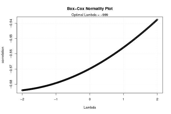
| Title produced by software | Box-Cox Normality Plot | ||||||||||||||||||||||||||||||||||||
| Date of computation | Tue, 16 Dec 2008 09:43:38 -0700 | ||||||||||||||||||||||||||||||||||||
| Cite this page as follows | Statistical Computations at FreeStatistics.org, Office for Research Development and Education, URL https://freestatistics.org/blog/index.php?v=date/2008/Dec/16/t1229445870sb3zq6nt3xafvoa.htm/, Retrieved Wed, 15 May 2024 11:11:44 +0000 | ||||||||||||||||||||||||||||||||||||
| Statistical Computations at FreeStatistics.org, Office for Research Development and Education, URL https://freestatistics.org/blog/index.php?pk=34029, Retrieved Wed, 15 May 2024 11:11:44 +0000 | |||||||||||||||||||||||||||||||||||||
| QR Codes: | |||||||||||||||||||||||||||||||||||||
|
| |||||||||||||||||||||||||||||||||||||
| Original text written by user: | |||||||||||||||||||||||||||||||||||||
| IsPrivate? | No (this computation is public) | ||||||||||||||||||||||||||||||||||||
| User-defined keywords | |||||||||||||||||||||||||||||||||||||
| Estimated Impact | 195 | ||||||||||||||||||||||||||||||||||||
Tree of Dependent Computations | |||||||||||||||||||||||||||||||||||||
| Family? (F = Feedback message, R = changed R code, M = changed R Module, P = changed Parameters, D = changed Data) | |||||||||||||||||||||||||||||||||||||
| - [Box-Cox Normality Plot] [paper box cox norm 1] [2007-12-01 09:46:32] [22f18fc6a98517db16300404be421f9a] - D [Box-Cox Normality Plot] [box cox normality...] [2008-12-16 16:40:09] [4ddbf81f78ea7c738951638c7e93f6ee] - D [Box-Cox Normality Plot] [box cox normality...] [2008-12-16 16:43:38] [e8f764b122b426f433a1e1038b457077] [Current] - D [Box-Cox Normality Plot] [box cox normality...] [2008-12-16 16:45:50] [4ddbf81f78ea7c738951638c7e93f6ee] | |||||||||||||||||||||||||||||||||||||
| Feedback Forum | |||||||||||||||||||||||||||||||||||||
Post a new message | |||||||||||||||||||||||||||||||||||||
Dataset | |||||||||||||||||||||||||||||||||||||
| Dataseries X: | |||||||||||||||||||||||||||||||||||||
9.4 9.5 9.1 9 9.3 9.9 9.8 9.4 8.3 8 8.5 10.4 11.1 10.9 9.9 9.2 9.2 9.5 9.6 9.5 9.1 8.9 9 10.1 10.3 10.2 9.6 9.2 9.3 9.4 9.4 9.2 9 9 9 9.8 10 9.9 9.3 9 9 9.1 9.1 9.1 9.2 8.8 8.3 8.4 8.1 7.8 7.9 7.9 8 7.9 7.5 7.2 6.9 6.6 6.7 7.3 | |||||||||||||||||||||||||||||||||||||
Tables (Output of Computation) | |||||||||||||||||||||||||||||||||||||
| |||||||||||||||||||||||||||||||||||||
Figures (Output of Computation) | |||||||||||||||||||||||||||||||||||||
Input Parameters & R Code | |||||||||||||||||||||||||||||||||||||
| Parameters (Session): | |||||||||||||||||||||||||||||||||||||
| Parameters (R input): | |||||||||||||||||||||||||||||||||||||
| R code (references can be found in the software module): | |||||||||||||||||||||||||||||||||||||
n <- length(x) | |||||||||||||||||||||||||||||||||||||