Repository of Reproducible Computations

Free Statistics

of Irreproducible Research!

Author's title

Author

*The author of this computation has been verified*

R Software Module

rwasp_autocorrelation.wasp

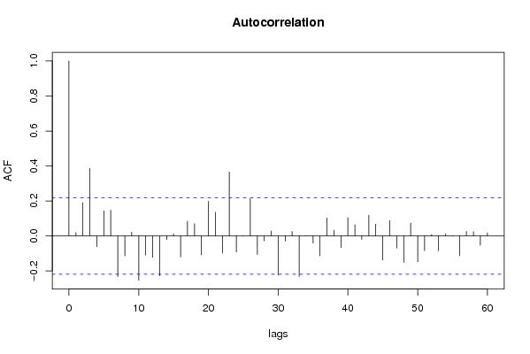
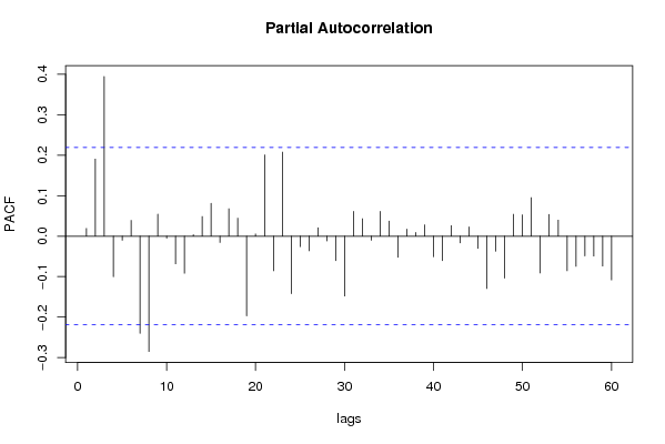
Title produced by software

(Partial) Autocorrelation Function

Date of computation

Tue, 16 Dec 2008 04:56:43 -0700

Cite this page as follows

Statistical Computations at FreeStatistics.org, Office for Research Development and Education, URL https://freestatistics.org/blog/index.php?v=date/2008/Dec/16/t12294286949xoyrftbx2r1qtj.htm/, Retrieved Wed, 15 May 2024 13:16:26 +0000

Statistical Computations at FreeStatistics.org, Office for Research Development and Education, URL https://freestatistics.org/blog/index.php?pk=33927, Retrieved Wed, 15 May 2024 13:16:26 +0000

QR Codes:

Paste this QR Code to cite your computation.

Original text written by user:

IsPrivate?

No (this computation is public)

User-defined keywords

Estimated Impact

222

Family? (F = Feedback message, R = changed R code, M = changed R Module, P = changed Parameters, D = changed Data)

-     [Univariate Data Series] [data set] [2008-12-01 19:54:57] [b98453cac15ba1066b407e146608df68]
F RMP   [(Partial) Autocorrelation Function] [ACF] [2008-12-08 11:23:44] [7173087adebe3e3a714c80ea2417b3eb]
-   PD    [(Partial) Autocorrelation Function] [(P) ACF - Totale ...] [2008-12-16 11:51:37] [29747f79f5beb5b2516e1271770ecb47]
-   PD        [(Partial) Autocorrelation Function] [(P) ACF - Totale ...] [2008-12-16 11:56:43] [c0a347e3519123f7eef62b705326dad9] [Current]

Feedback Forum

Post a new message

Dataseries X:

Download CSV

Histogram

Boxplots

Summary of computational transaction
Raw Input	view raw input (R code)
Raw Output	view raw output of R engine
Computing time	1 seconds
R Server	'Gwilym Jenkins' @ 72.249.127.135

\begin{tabular}{lllllllll}
\hline
Summary of computational transaction \tabularnewline
Raw Input & view raw input (R code)  \tabularnewline
Raw Output & view raw output of R engine  \tabularnewline
Computing time & 1 seconds \tabularnewline
R Server & 'Gwilym Jenkins' @ 72.249.127.135 \tabularnewline
\hline
\end{tabular}
%Source: https://freestatistics.org/blog/index.php?pk=33927&T=0

[TABLE]
[ROW][C]Summary of computational transaction[/C][/ROW]
[ROW][C]Raw Input[/C][C]view raw input (R code) [/C][/ROW]
[ROW][C]Raw Output[/C][C]view raw output of R engine [/C][/ROW]
[ROW][C]Computing time[/C][C]1 seconds[/C][/ROW]
[ROW][C]R Server[/C][C]'Gwilym Jenkins' @ 72.249.127.135[/C][/ROW]
[/TABLE]
Source: https://freestatistics.org/blog/index.php?pk=33927&T=0

Globally Unique Identifier (entire table): ba.freestatistics.org/blog/index.php?pk=33927&T=0

As an alternative you can also use a QR Code:

The GUIDs for individual cells are displayed in the table below:

Summary of computational transaction
Raw Input	view raw input (R code)
Raw Output	view raw output of R engine
Computing time	1 seconds
R Server	'Gwilym Jenkins' @ 72.249.127.135

Autocorrelation Function
Time lag k	ACF(k)	T-STAT	P-value
1	0.019142	0.1712	0.432245
2	0.19063	1.705	0.046034
3	0.386521	3.4572	0.000439
4	-0.061837	-0.5531	0.290873
5	0.143601	1.2844	0.101354
6	0.147155	1.3162	0.095934
7	-0.231903	-2.0742	0.020638
8	-0.113527	-1.0154	0.156485
9	0.021626	0.1934	0.423556
10	-0.253361	-2.2661	0.013072
11	-0.109904	-0.983	0.164283
12	-0.121813	-1.0895	0.139597
13	-0.228132	-2.0405	0.022301
14	-0.020832	-0.1863	0.426329
15	0.012123	0.1084	0.456962
16	-0.119797	-1.0715	0.143584
17	0.08342	0.7461	0.228887
18	0.069662	0.6231	0.267504
19	-0.108677	-0.972	0.166982
20	0.198141	1.7722	0.040082
21	0.135332	1.2104	0.114836
22	-0.098096	-0.8774	0.191448
23	0.36586	3.2724	0.000788
24	-0.092232	-0.825	0.205926
25	-0.001122	-0.01	0.496008
26	0.213381	1.9085	0.029954
27	-0.105611	-0.9446	0.173849
28	-0.027794	-0.2486	0.402156
29	0.028546	0.2553	0.399565
30	-0.223697	-2.0008	0.024402
31	-0.028964	-0.2591	0.398127
32	0.025381	0.227	0.410497
33	-0.232221	-2.077	0.020503
34	0.000444	0.004	0.49842
35	-0.040941	-0.3662	0.357597
36	-0.113808	-1.0179	0.15589
37	0.102314	0.9151	0.181438
38	0.033088	0.2959	0.384018
39	-0.067039	-0.5996	0.275228
40	0.104802	0.9374	0.175692
41	0.063387	0.567	0.286167
42	-0.019783	-0.1769	0.430001
43	0.118256	1.0577	0.146686
44	0.067354	0.6024	0.274295
45	-0.137542	-1.2302	0.111111
46	0.087555	0.7831	0.217936
47	-0.068895	-0.6162	0.269751
48	-0.151509	-1.3551	0.089594
49	0.073957	0.6615	0.255099
50	-0.147932	-1.3231	0.094778
51	-0.083832	-0.7498	0.227784
52	0.008525	0.0763	0.469705
53	-0.084645	-0.7571	0.225611
54	0.011495	0.1028	0.459185
55	-0.001236	-0.0111	0.495605
56	-0.112966	-1.0104	0.157676
57	0.026105	0.2335	0.407988
58	0.025022	0.2238	0.411741
59	-0.053129	-0.4752	0.317969
60	0.016907	0.1512	0.44009

\begin{tabular}{lllllllll}
\hline
Autocorrelation Function \tabularnewline
Time lag k & ACF(k) & T-STAT & P-value \tabularnewline
1 & 0.019142 & 0.1712 & 0.432245 \tabularnewline
2 & 0.19063 & 1.705 & 0.046034 \tabularnewline
3 & 0.386521 & 3.4572 & 0.000439 \tabularnewline
4 & -0.061837 & -0.5531 & 0.290873 \tabularnewline
5 & 0.143601 & 1.2844 & 0.101354 \tabularnewline
6 & 0.147155 & 1.3162 & 0.095934 \tabularnewline
7 & -0.231903 & -2.0742 & 0.020638 \tabularnewline
8 & -0.113527 & -1.0154 & 0.156485 \tabularnewline
9 & 0.021626 & 0.1934 & 0.423556 \tabularnewline
10 & -0.253361 & -2.2661 & 0.013072 \tabularnewline
11 & -0.109904 & -0.983 & 0.164283 \tabularnewline
12 & -0.121813 & -1.0895 & 0.139597 \tabularnewline
13 & -0.228132 & -2.0405 & 0.022301 \tabularnewline
14 & -0.020832 & -0.1863 & 0.426329 \tabularnewline
15 & 0.012123 & 0.1084 & 0.456962 \tabularnewline
16 & -0.119797 & -1.0715 & 0.143584 \tabularnewline
17 & 0.08342 & 0.7461 & 0.228887 \tabularnewline
18 & 0.069662 & 0.6231 & 0.267504 \tabularnewline
19 & -0.108677 & -0.972 & 0.166982 \tabularnewline
20 & 0.198141 & 1.7722 & 0.040082 \tabularnewline
21 & 0.135332 & 1.2104 & 0.114836 \tabularnewline
22 & -0.098096 & -0.8774 & 0.191448 \tabularnewline
23 & 0.36586 & 3.2724 & 0.000788 \tabularnewline
24 & -0.092232 & -0.825 & 0.205926 \tabularnewline
25 & -0.001122 & -0.01 & 0.496008 \tabularnewline
26 & 0.213381 & 1.9085 & 0.029954 \tabularnewline
27 & -0.105611 & -0.9446 & 0.173849 \tabularnewline
28 & -0.027794 & -0.2486 & 0.402156 \tabularnewline
29 & 0.028546 & 0.2553 & 0.399565 \tabularnewline
30 & -0.223697 & -2.0008 & 0.024402 \tabularnewline
31 & -0.028964 & -0.2591 & 0.398127 \tabularnewline
32 & 0.025381 & 0.227 & 0.410497 \tabularnewline
33 & -0.232221 & -2.077 & 0.020503 \tabularnewline
34 & 0.000444 & 0.004 & 0.49842 \tabularnewline
35 & -0.040941 & -0.3662 & 0.357597 \tabularnewline
36 & -0.113808 & -1.0179 & 0.15589 \tabularnewline
37 & 0.102314 & 0.9151 & 0.181438 \tabularnewline
38 & 0.033088 & 0.2959 & 0.384018 \tabularnewline
39 & -0.067039 & -0.5996 & 0.275228 \tabularnewline
40 & 0.104802 & 0.9374 & 0.175692 \tabularnewline
41 & 0.063387 & 0.567 & 0.286167 \tabularnewline
42 & -0.019783 & -0.1769 & 0.430001 \tabularnewline
43 & 0.118256 & 1.0577 & 0.146686 \tabularnewline
44 & 0.067354 & 0.6024 & 0.274295 \tabularnewline
45 & -0.137542 & -1.2302 & 0.111111 \tabularnewline
46 & 0.087555 & 0.7831 & 0.217936 \tabularnewline
47 & -0.068895 & -0.6162 & 0.269751 \tabularnewline
48 & -0.151509 & -1.3551 & 0.089594 \tabularnewline
49 & 0.073957 & 0.6615 & 0.255099 \tabularnewline
50 & -0.147932 & -1.3231 & 0.094778 \tabularnewline
51 & -0.083832 & -0.7498 & 0.227784 \tabularnewline
52 & 0.008525 & 0.0763 & 0.469705 \tabularnewline
53 & -0.084645 & -0.7571 & 0.225611 \tabularnewline
54 & 0.011495 & 0.1028 & 0.459185 \tabularnewline
55 & -0.001236 & -0.0111 & 0.495605 \tabularnewline
56 & -0.112966 & -1.0104 & 0.157676 \tabularnewline
57 & 0.026105 & 0.2335 & 0.407988 \tabularnewline
58 & 0.025022 & 0.2238 & 0.411741 \tabularnewline
59 & -0.053129 & -0.4752 & 0.317969 \tabularnewline
60 & 0.016907 & 0.1512 & 0.44009 \tabularnewline
\hline
\end{tabular}
%Source: https://freestatistics.org/blog/index.php?pk=33927&T=1

[TABLE]
[ROW][C]Autocorrelation Function[/C][/ROW]
[ROW][C]Time lag k[/C][C]ACF(k)[/C][C]T-STAT[/C][C]P-value[/C][/ROW]
[ROW][C]1[/C][C]0.019142[/C][C]0.1712[/C][C]0.432245[/C][/ROW]
[ROW][C]2[/C][C]0.19063[/C][C]1.705[/C][C]0.046034[/C][/ROW]
[ROW][C]3[/C][C]0.386521[/C][C]3.4572[/C][C]0.000439[/C][/ROW]
[ROW][C]4[/C][C]-0.061837[/C][C]-0.5531[/C][C]0.290873[/C][/ROW]
[ROW][C]5[/C][C]0.143601[/C][C]1.2844[/C][C]0.101354[/C][/ROW]
[ROW][C]6[/C][C]0.147155[/C][C]1.3162[/C][C]0.095934[/C][/ROW]
[ROW][C]7[/C][C]-0.231903[/C][C]-2.0742[/C][C]0.020638[/C][/ROW]
[ROW][C]8[/C][C]-0.113527[/C][C]-1.0154[/C][C]0.156485[/C][/ROW]
[ROW][C]9[/C][C]0.021626[/C][C]0.1934[/C][C]0.423556[/C][/ROW]
[ROW][C]10[/C][C]-0.253361[/C][C]-2.2661[/C][C]0.013072[/C][/ROW]
[ROW][C]11[/C][C]-0.109904[/C][C]-0.983[/C][C]0.164283[/C][/ROW]
[ROW][C]12[/C][C]-0.121813[/C][C]-1.0895[/C][C]0.139597[/C][/ROW]
[ROW][C]13[/C][C]-0.228132[/C][C]-2.0405[/C][C]0.022301[/C][/ROW]
[ROW][C]14[/C][C]-0.020832[/C][C]-0.1863[/C][C]0.426329[/C][/ROW]
[ROW][C]15[/C][C]0.012123[/C][C]0.1084[/C][C]0.456962[/C][/ROW]
[ROW][C]16[/C][C]-0.119797[/C][C]-1.0715[/C][C]0.143584[/C][/ROW]
[ROW][C]17[/C][C]0.08342[/C][C]0.7461[/C][C]0.228887[/C][/ROW]
[ROW][C]18[/C][C]0.069662[/C][C]0.6231[/C][C]0.267504[/C][/ROW]
[ROW][C]19[/C][C]-0.108677[/C][C]-0.972[/C][C]0.166982[/C][/ROW]
[ROW][C]20[/C][C]0.198141[/C][C]1.7722[/C][C]0.040082[/C][/ROW]
[ROW][C]21[/C][C]0.135332[/C][C]1.2104[/C][C]0.114836[/C][/ROW]
[ROW][C]22[/C][C]-0.098096[/C][C]-0.8774[/C][C]0.191448[/C][/ROW]
[ROW][C]23[/C][C]0.36586[/C][C]3.2724[/C][C]0.000788[/C][/ROW]
[ROW][C]24[/C][C]-0.092232[/C][C]-0.825[/C][C]0.205926[/C][/ROW]
[ROW][C]25[/C][C]-0.001122[/C][C]-0.01[/C][C]0.496008[/C][/ROW]
[ROW][C]26[/C][C]0.213381[/C][C]1.9085[/C][C]0.029954[/C][/ROW]
[ROW][C]27[/C][C]-0.105611[/C][C]-0.9446[/C][C]0.173849[/C][/ROW]
[ROW][C]28[/C][C]-0.027794[/C][C]-0.2486[/C][C]0.402156[/C][/ROW]
[ROW][C]29[/C][C]0.028546[/C][C]0.2553[/C][C]0.399565[/C][/ROW]
[ROW][C]30[/C][C]-0.223697[/C][C]-2.0008[/C][C]0.024402[/C][/ROW]
[ROW][C]31[/C][C]-0.028964[/C][C]-0.2591[/C][C]0.398127[/C][/ROW]
[ROW][C]32[/C][C]0.025381[/C][C]0.227[/C][C]0.410497[/C][/ROW]
[ROW][C]33[/C][C]-0.232221[/C][C]-2.077[/C][C]0.020503[/C][/ROW]
[ROW][C]34[/C][C]0.000444[/C][C]0.004[/C][C]0.49842[/C][/ROW]
[ROW][C]35[/C][C]-0.040941[/C][C]-0.3662[/C][C]0.357597[/C][/ROW]
[ROW][C]36[/C][C]-0.113808[/C][C]-1.0179[/C][C]0.15589[/C][/ROW]
[ROW][C]37[/C][C]0.102314[/C][C]0.9151[/C][C]0.181438[/C][/ROW]
[ROW][C]38[/C][C]0.033088[/C][C]0.2959[/C][C]0.384018[/C][/ROW]
[ROW][C]39[/C][C]-0.067039[/C][C]-0.5996[/C][C]0.275228[/C][/ROW]
[ROW][C]40[/C][C]0.104802[/C][C]0.9374[/C][C]0.175692[/C][/ROW]
[ROW][C]41[/C][C]0.063387[/C][C]0.567[/C][C]0.286167[/C][/ROW]
[ROW][C]42[/C][C]-0.019783[/C][C]-0.1769[/C][C]0.430001[/C][/ROW]
[ROW][C]43[/C][C]0.118256[/C][C]1.0577[/C][C]0.146686[/C][/ROW]
[ROW][C]44[/C][C]0.067354[/C][C]0.6024[/C][C]0.274295[/C][/ROW]
[ROW][C]45[/C][C]-0.137542[/C][C]-1.2302[/C][C]0.111111[/C][/ROW]
[ROW][C]46[/C][C]0.087555[/C][C]0.7831[/C][C]0.217936[/C][/ROW]
[ROW][C]47[/C][C]-0.068895[/C][C]-0.6162[/C][C]0.269751[/C][/ROW]
[ROW][C]48[/C][C]-0.151509[/C][C]-1.3551[/C][C]0.089594[/C][/ROW]
[ROW][C]49[/C][C]0.073957[/C][C]0.6615[/C][C]0.255099[/C][/ROW]
[ROW][C]50[/C][C]-0.147932[/C][C]-1.3231[/C][C]0.094778[/C][/ROW]
[ROW][C]51[/C][C]-0.083832[/C][C]-0.7498[/C][C]0.227784[/C][/ROW]
[ROW][C]52[/C][C]0.008525[/C][C]0.0763[/C][C]0.469705[/C][/ROW]
[ROW][C]53[/C][C]-0.084645[/C][C]-0.7571[/C][C]0.225611[/C][/ROW]
[ROW][C]54[/C][C]0.011495[/C][C]0.1028[/C][C]0.459185[/C][/ROW]
[ROW][C]55[/C][C]-0.001236[/C][C]-0.0111[/C][C]0.495605[/C][/ROW]
[ROW][C]56[/C][C]-0.112966[/C][C]-1.0104[/C][C]0.157676[/C][/ROW]
[ROW][C]57[/C][C]0.026105[/C][C]0.2335[/C][C]0.407988[/C][/ROW]
[ROW][C]58[/C][C]0.025022[/C][C]0.2238[/C][C]0.411741[/C][/ROW]
[ROW][C]59[/C][C]-0.053129[/C][C]-0.4752[/C][C]0.317969[/C][/ROW]
[ROW][C]60[/C][C]0.016907[/C][C]0.1512[/C][C]0.44009[/C][/ROW]
[/TABLE]
Source: https://freestatistics.org/blog/index.php?pk=33927&T=1

Globally Unique Identifier (entire table): ba.freestatistics.org/blog/index.php?pk=33927&T=1

As an alternative you can also use a QR Code:

The GUIDs for individual cells are displayed in the table below:

Autocorrelation Function
Time lag k	ACF(k)	T-STAT	P-value
1	0.019142	0.1712	0.432245
2	0.19063	1.705	0.046034
3	0.386521	3.4572	0.000439
4	-0.061837	-0.5531	0.290873
5	0.143601	1.2844	0.101354
6	0.147155	1.3162	0.095934
7	-0.231903	-2.0742	0.020638
8	-0.113527	-1.0154	0.156485
9	0.021626	0.1934	0.423556
10	-0.253361	-2.2661	0.013072
11	-0.109904	-0.983	0.164283
12	-0.121813	-1.0895	0.139597
13	-0.228132	-2.0405	0.022301
14	-0.020832	-0.1863	0.426329
15	0.012123	0.1084	0.456962
16	-0.119797	-1.0715	0.143584
17	0.08342	0.7461	0.228887
18	0.069662	0.6231	0.267504
19	-0.108677	-0.972	0.166982
20	0.198141	1.7722	0.040082
21	0.135332	1.2104	0.114836
22	-0.098096	-0.8774	0.191448
23	0.36586	3.2724	0.000788
24	-0.092232	-0.825	0.205926
25	-0.001122	-0.01	0.496008
26	0.213381	1.9085	0.029954
27	-0.105611	-0.9446	0.173849
28	-0.027794	-0.2486	0.402156
29	0.028546	0.2553	0.399565
30	-0.223697	-2.0008	0.024402
31	-0.028964	-0.2591	0.398127
32	0.025381	0.227	0.410497
33	-0.232221	-2.077	0.020503
34	0.000444	0.004	0.49842
35	-0.040941	-0.3662	0.357597
36	-0.113808	-1.0179	0.15589
37	0.102314	0.9151	0.181438
38	0.033088	0.2959	0.384018
39	-0.067039	-0.5996	0.275228
40	0.104802	0.9374	0.175692
41	0.063387	0.567	0.286167
42	-0.019783	-0.1769	0.430001
43	0.118256	1.0577	0.146686
44	0.067354	0.6024	0.274295
45	-0.137542	-1.2302	0.111111
46	0.087555	0.7831	0.217936
47	-0.068895	-0.6162	0.269751
48	-0.151509	-1.3551	0.089594
49	0.073957	0.6615	0.255099
50	-0.147932	-1.3231	0.094778
51	-0.083832	-0.7498	0.227784
52	0.008525	0.0763	0.469705
53	-0.084645	-0.7571	0.225611
54	0.011495	0.1028	0.459185
55	-0.001236	-0.0111	0.495605
56	-0.112966	-1.0104	0.157676
57	0.026105	0.2335	0.407988
58	0.025022	0.2238	0.411741
59	-0.053129	-0.4752	0.317969
60	0.016907	0.1512	0.44009

Partial Autocorrelation Function
Time lag k	PACF(k)	T-STAT	P-value
1	0.019142	0.1712	0.432245
2	0.190333	1.7024	0.046283
3	0.394349	3.5272	0.000349
4	-0.100151	-0.8958	0.18653
5	-0.010053	-0.0899	0.464289
6	0.038954	0.3484	0.364223
7	-0.239973	-2.1464	0.017436
8	-0.284926	-2.5485	0.006367
9	0.05434	0.486	0.314136
10	-0.004913	-0.0439	0.48253
11	-0.068276	-0.6107	0.271572
12	-0.091775	-0.8209	0.207082
13	0.00369	0.033	0.486876
14	0.048566	0.4344	0.332587
15	0.081124	0.7256	0.235102
16	-0.015588	-0.1394	0.444733
17	0.067779	0.6062	0.273039
18	0.044262	0.3959	0.34662
19	-0.196771	-1.76	0.041117
20	0.005162	0.0462	0.481646
21	0.200773	1.7958	0.038154
22	-0.085364	-0.7635	0.2237
23	0.207564	1.8565	0.033532
24	-0.142026	-1.2703	0.103826
25	-0.025866	-0.2314	0.408817
26	-0.036265	-0.3244	0.373253
27	0.020755	0.1856	0.4266
28	-0.011948	-0.1069	0.457582
29	-0.060388	-0.5401	0.295304
30	-0.148071	-1.3244	0.094573
31	0.061199	0.5474	0.29282
32	0.043021	0.3848	0.350705
33	-0.010092	-0.0903	0.464151
34	0.061061	0.5461	0.293243
35	0.037227	0.333	0.370016
36	-0.052299	-0.4678	0.320607
37	0.017464	0.1562	0.438135
38	0.008972	0.0802	0.468121
39	0.027825	0.2489	0.402047
40	-0.050831	-0.4546	0.325298
41	-0.060664	-0.5426	0.294458
42	0.025816	0.2309	0.408989
43	-0.016531	-0.1479	0.441415
44	0.022717	0.2032	0.419754
45	-0.030259	-0.2706	0.39368
46	-0.129548	-1.1587	0.125011
47	-0.037337	-0.334	0.369645
48	-0.103772	-0.9282	0.178057
49	0.053905	0.4821	0.315511
50	0.05252	0.4698	0.319904
51	0.094969	0.8494	0.199088
52	-0.090878	-0.8128	0.209361
53	0.053543	0.4789	0.316657
54	0.039471	0.353	0.362494
55	-0.085409	-0.7639	0.223582
56	-0.074478	-0.6661	0.253616
57	-0.048954	-0.4379	0.331336
58	-0.049139	-0.4395	0.330739
59	-0.073976	-0.6617	0.255045
60	-0.108018	-0.9661	0.168442

\begin{tabular}{lllllllll}
\hline
Partial Autocorrelation Function \tabularnewline
Time lag k & PACF(k) & T-STAT & P-value \tabularnewline
1 & 0.019142 & 0.1712 & 0.432245 \tabularnewline
2 & 0.190333 & 1.7024 & 0.046283 \tabularnewline
3 & 0.394349 & 3.5272 & 0.000349 \tabularnewline
4 & -0.100151 & -0.8958 & 0.18653 \tabularnewline
5 & -0.010053 & -0.0899 & 0.464289 \tabularnewline
6 & 0.038954 & 0.3484 & 0.364223 \tabularnewline
7 & -0.239973 & -2.1464 & 0.017436 \tabularnewline
8 & -0.284926 & -2.5485 & 0.006367 \tabularnewline
9 & 0.05434 & 0.486 & 0.314136 \tabularnewline
10 & -0.004913 & -0.0439 & 0.48253 \tabularnewline
11 & -0.068276 & -0.6107 & 0.271572 \tabularnewline
12 & -0.091775 & -0.8209 & 0.207082 \tabularnewline
13 & 0.00369 & 0.033 & 0.486876 \tabularnewline
14 & 0.048566 & 0.4344 & 0.332587 \tabularnewline
15 & 0.081124 & 0.7256 & 0.235102 \tabularnewline
16 & -0.015588 & -0.1394 & 0.444733 \tabularnewline
17 & 0.067779 & 0.6062 & 0.273039 \tabularnewline
18 & 0.044262 & 0.3959 & 0.34662 \tabularnewline
19 & -0.196771 & -1.76 & 0.041117 \tabularnewline
20 & 0.005162 & 0.0462 & 0.481646 \tabularnewline
21 & 0.200773 & 1.7958 & 0.038154 \tabularnewline
22 & -0.085364 & -0.7635 & 0.2237 \tabularnewline
23 & 0.207564 & 1.8565 & 0.033532 \tabularnewline
24 & -0.142026 & -1.2703 & 0.103826 \tabularnewline
25 & -0.025866 & -0.2314 & 0.408817 \tabularnewline
26 & -0.036265 & -0.3244 & 0.373253 \tabularnewline
27 & 0.020755 & 0.1856 & 0.4266 \tabularnewline
28 & -0.011948 & -0.1069 & 0.457582 \tabularnewline
29 & -0.060388 & -0.5401 & 0.295304 \tabularnewline
30 & -0.148071 & -1.3244 & 0.094573 \tabularnewline
31 & 0.061199 & 0.5474 & 0.29282 \tabularnewline
32 & 0.043021 & 0.3848 & 0.350705 \tabularnewline
33 & -0.010092 & -0.0903 & 0.464151 \tabularnewline
34 & 0.061061 & 0.5461 & 0.293243 \tabularnewline
35 & 0.037227 & 0.333 & 0.370016 \tabularnewline
36 & -0.052299 & -0.4678 & 0.320607 \tabularnewline
37 & 0.017464 & 0.1562 & 0.438135 \tabularnewline
38 & 0.008972 & 0.0802 & 0.468121 \tabularnewline
39 & 0.027825 & 0.2489 & 0.402047 \tabularnewline
40 & -0.050831 & -0.4546 & 0.325298 \tabularnewline
41 & -0.060664 & -0.5426 & 0.294458 \tabularnewline
42 & 0.025816 & 0.2309 & 0.408989 \tabularnewline
43 & -0.016531 & -0.1479 & 0.441415 \tabularnewline
44 & 0.022717 & 0.2032 & 0.419754 \tabularnewline
45 & -0.030259 & -0.2706 & 0.39368 \tabularnewline
46 & -0.129548 & -1.1587 & 0.125011 \tabularnewline
47 & -0.037337 & -0.334 & 0.369645 \tabularnewline
48 & -0.103772 & -0.9282 & 0.178057 \tabularnewline
49 & 0.053905 & 0.4821 & 0.315511 \tabularnewline
50 & 0.05252 & 0.4698 & 0.319904 \tabularnewline
51 & 0.094969 & 0.8494 & 0.199088 \tabularnewline
52 & -0.090878 & -0.8128 & 0.209361 \tabularnewline
53 & 0.053543 & 0.4789 & 0.316657 \tabularnewline
54 & 0.039471 & 0.353 & 0.362494 \tabularnewline
55 & -0.085409 & -0.7639 & 0.223582 \tabularnewline
56 & -0.074478 & -0.6661 & 0.253616 \tabularnewline
57 & -0.048954 & -0.4379 & 0.331336 \tabularnewline
58 & -0.049139 & -0.4395 & 0.330739 \tabularnewline
59 & -0.073976 & -0.6617 & 0.255045 \tabularnewline
60 & -0.108018 & -0.9661 & 0.168442 \tabularnewline
\hline
\end{tabular}
%Source: https://freestatistics.org/blog/index.php?pk=33927&T=2

[TABLE]
[ROW][C]Partial Autocorrelation Function[/C][/ROW]
[ROW][C]Time lag k[/C][C]PACF(k)[/C][C]T-STAT[/C][C]P-value[/C][/ROW]
[ROW][C]1[/C][C]0.019142[/C][C]0.1712[/C][C]0.432245[/C][/ROW]
[ROW][C]2[/C][C]0.190333[/C][C]1.7024[/C][C]0.046283[/C][/ROW]
[ROW][C]3[/C][C]0.394349[/C][C]3.5272[/C][C]0.000349[/C][/ROW]
[ROW][C]4[/C][C]-0.100151[/C][C]-0.8958[/C][C]0.18653[/C][/ROW]
[ROW][C]5[/C][C]-0.010053[/C][C]-0.0899[/C][C]0.464289[/C][/ROW]
[ROW][C]6[/C][C]0.038954[/C][C]0.3484[/C][C]0.364223[/C][/ROW]
[ROW][C]7[/C][C]-0.239973[/C][C]-2.1464[/C][C]0.017436[/C][/ROW]
[ROW][C]8[/C][C]-0.284926[/C][C]-2.5485[/C][C]0.006367[/C][/ROW]
[ROW][C]9[/C][C]0.05434[/C][C]0.486[/C][C]0.314136[/C][/ROW]
[ROW][C]10[/C][C]-0.004913[/C][C]-0.0439[/C][C]0.48253[/C][/ROW]
[ROW][C]11[/C][C]-0.068276[/C][C]-0.6107[/C][C]0.271572[/C][/ROW]
[ROW][C]12[/C][C]-0.091775[/C][C]-0.8209[/C][C]0.207082[/C][/ROW]
[ROW][C]13[/C][C]0.00369[/C][C]0.033[/C][C]0.486876[/C][/ROW]
[ROW][C]14[/C][C]0.048566[/C][C]0.4344[/C][C]0.332587[/C][/ROW]
[ROW][C]15[/C][C]0.081124[/C][C]0.7256[/C][C]0.235102[/C][/ROW]
[ROW][C]16[/C][C]-0.015588[/C][C]-0.1394[/C][C]0.444733[/C][/ROW]
[ROW][C]17[/C][C]0.067779[/C][C]0.6062[/C][C]0.273039[/C][/ROW]
[ROW][C]18[/C][C]0.044262[/C][C]0.3959[/C][C]0.34662[/C][/ROW]
[ROW][C]19[/C][C]-0.196771[/C][C]-1.76[/C][C]0.041117[/C][/ROW]
[ROW][C]20[/C][C]0.005162[/C][C]0.0462[/C][C]0.481646[/C][/ROW]
[ROW][C]21[/C][C]0.200773[/C][C]1.7958[/C][C]0.038154[/C][/ROW]
[ROW][C]22[/C][C]-0.085364[/C][C]-0.7635[/C][C]0.2237[/C][/ROW]
[ROW][C]23[/C][C]0.207564[/C][C]1.8565[/C][C]0.033532[/C][/ROW]
[ROW][C]24[/C][C]-0.142026[/C][C]-1.2703[/C][C]0.103826[/C][/ROW]
[ROW][C]25[/C][C]-0.025866[/C][C]-0.2314[/C][C]0.408817[/C][/ROW]
[ROW][C]26[/C][C]-0.036265[/C][C]-0.3244[/C][C]0.373253[/C][/ROW]
[ROW][C]27[/C][C]0.020755[/C][C]0.1856[/C][C]0.4266[/C][/ROW]
[ROW][C]28[/C][C]-0.011948[/C][C]-0.1069[/C][C]0.457582[/C][/ROW]
[ROW][C]29[/C][C]-0.060388[/C][C]-0.5401[/C][C]0.295304[/C][/ROW]
[ROW][C]30[/C][C]-0.148071[/C][C]-1.3244[/C][C]0.094573[/C][/ROW]
[ROW][C]31[/C][C]0.061199[/C][C]0.5474[/C][C]0.29282[/C][/ROW]
[ROW][C]32[/C][C]0.043021[/C][C]0.3848[/C][C]0.350705[/C][/ROW]
[ROW][C]33[/C][C]-0.010092[/C][C]-0.0903[/C][C]0.464151[/C][/ROW]
[ROW][C]34[/C][C]0.061061[/C][C]0.5461[/C][C]0.293243[/C][/ROW]
[ROW][C]35[/C][C]0.037227[/C][C]0.333[/C][C]0.370016[/C][/ROW]
[ROW][C]36[/C][C]-0.052299[/C][C]-0.4678[/C][C]0.320607[/C][/ROW]
[ROW][C]37[/C][C]0.017464[/C][C]0.1562[/C][C]0.438135[/C][/ROW]
[ROW][C]38[/C][C]0.008972[/C][C]0.0802[/C][C]0.468121[/C][/ROW]
[ROW][C]39[/C][C]0.027825[/C][C]0.2489[/C][C]0.402047[/C][/ROW]
[ROW][C]40[/C][C]-0.050831[/C][C]-0.4546[/C][C]0.325298[/C][/ROW]
[ROW][C]41[/C][C]-0.060664[/C][C]-0.5426[/C][C]0.294458[/C][/ROW]
[ROW][C]42[/C][C]0.025816[/C][C]0.2309[/C][C]0.408989[/C][/ROW]
[ROW][C]43[/C][C]-0.016531[/C][C]-0.1479[/C][C]0.441415[/C][/ROW]
[ROW][C]44[/C][C]0.022717[/C][C]0.2032[/C][C]0.419754[/C][/ROW]
[ROW][C]45[/C][C]-0.030259[/C][C]-0.2706[/C][C]0.39368[/C][/ROW]
[ROW][C]46[/C][C]-0.129548[/C][C]-1.1587[/C][C]0.125011[/C][/ROW]
[ROW][C]47[/C][C]-0.037337[/C][C]-0.334[/C][C]0.369645[/C][/ROW]
[ROW][C]48[/C][C]-0.103772[/C][C]-0.9282[/C][C]0.178057[/C][/ROW]
[ROW][C]49[/C][C]0.053905[/C][C]0.4821[/C][C]0.315511[/C][/ROW]
[ROW][C]50[/C][C]0.05252[/C][C]0.4698[/C][C]0.319904[/C][/ROW]
[ROW][C]51[/C][C]0.094969[/C][C]0.8494[/C][C]0.199088[/C][/ROW]
[ROW][C]52[/C][C]-0.090878[/C][C]-0.8128[/C][C]0.209361[/C][/ROW]
[ROW][C]53[/C][C]0.053543[/C][C]0.4789[/C][C]0.316657[/C][/ROW]
[ROW][C]54[/C][C]0.039471[/C][C]0.353[/C][C]0.362494[/C][/ROW]
[ROW][C]55[/C][C]-0.085409[/C][C]-0.7639[/C][C]0.223582[/C][/ROW]
[ROW][C]56[/C][C]-0.074478[/C][C]-0.6661[/C][C]0.253616[/C][/ROW]
[ROW][C]57[/C][C]-0.048954[/C][C]-0.4379[/C][C]0.331336[/C][/ROW]
[ROW][C]58[/C][C]-0.049139[/C][C]-0.4395[/C][C]0.330739[/C][/ROW]
[ROW][C]59[/C][C]-0.073976[/C][C]-0.6617[/C][C]0.255045[/C][/ROW]
[ROW][C]60[/C][C]-0.108018[/C][C]-0.9661[/C][C]0.168442[/C][/ROW]
[/TABLE]
Source: https://freestatistics.org/blog/index.php?pk=33927&T=2

Globally Unique Identifier (entire table): ba.freestatistics.org/blog/index.php?pk=33927&T=2

As an alternative you can also use a QR Code:

The GUIDs for individual cells are displayed in the table below:

Partial Autocorrelation Function
Time lag k	PACF(k)	T-STAT	P-value
1	0.019142	0.1712	0.432245
2	0.190333	1.7024	0.046283
3	0.394349	3.5272	0.000349
4	-0.100151	-0.8958	0.18653
5	-0.010053	-0.0899	0.464289
6	0.038954	0.3484	0.364223
7	-0.239973	-2.1464	0.017436
8	-0.284926	-2.5485	0.006367
9	0.05434	0.486	0.314136
10	-0.004913	-0.0439	0.48253
11	-0.068276	-0.6107	0.271572
12	-0.091775	-0.8209	0.207082
13	0.00369	0.033	0.486876
14	0.048566	0.4344	0.332587
15	0.081124	0.7256	0.235102
16	-0.015588	-0.1394	0.444733
17	0.067779	0.6062	0.273039
18	0.044262	0.3959	0.34662
19	-0.196771	-1.76	0.041117
20	0.005162	0.0462	0.481646
21	0.200773	1.7958	0.038154
22	-0.085364	-0.7635	0.2237
23	0.207564	1.8565	0.033532
24	-0.142026	-1.2703	0.103826
25	-0.025866	-0.2314	0.408817
26	-0.036265	-0.3244	0.373253
27	0.020755	0.1856	0.4266
28	-0.011948	-0.1069	0.457582
29	-0.060388	-0.5401	0.295304
30	-0.148071	-1.3244	0.094573
31	0.061199	0.5474	0.29282
32	0.043021	0.3848	0.350705
33	-0.010092	-0.0903	0.464151
34	0.061061	0.5461	0.293243
35	0.037227	0.333	0.370016
36	-0.052299	-0.4678	0.320607
37	0.017464	0.1562	0.438135
38	0.008972	0.0802	0.468121
39	0.027825	0.2489	0.402047
40	-0.050831	-0.4546	0.325298
41	-0.060664	-0.5426	0.294458
42	0.025816	0.2309	0.408989
43	-0.016531	-0.1479	0.441415
44	0.022717	0.2032	0.419754
45	-0.030259	-0.2706	0.39368
46	-0.129548	-1.1587	0.125011
47	-0.037337	-0.334	0.369645
48	-0.103772	-0.9282	0.178057
49	0.053905	0.4821	0.315511
50	0.05252	0.4698	0.319904
51	0.094969	0.8494	0.199088
52	-0.090878	-0.8128	0.209361
53	0.053543	0.4789	0.316657
54	0.039471	0.353	0.362494
55	-0.085409	-0.7639	0.223582
56	-0.074478	-0.6661	0.253616
57	-0.048954	-0.4379	0.331336
58	-0.049139	-0.4395	0.330739
59	-0.073976	-0.6617	0.255045
60	-0.108018	-0.9661	0.168442

Figure 1

PNG link

Postscript link

PDF link

Figure 2

PNG link

Postscript link

PDF link

Parameters (Session):

par1 = 60 ; par2 = 1 ; par3 = 0 ; par4 = 1 ; par5 = 12 ;

Parameters (R input):

par1 = 60 ; par2 = 1 ; par3 = 0 ; par4 = 1 ; par5 = 12 ;

R code (references can be found in the software module):

if (par1 == 'Default') {
par1 = 10*log10(length(x))
} else {
par1 <- as.numeric(par1)
}
par2 <- as.numeric(par2)
par3 <- as.numeric(par3)
par4 <- as.numeric(par4)
par5 <- as.numeric(par5)
if (par2 == 0) {
x <- log(x)
} else {
x <- (x ^ par2 - 1) / par2
}
if (par3 > 0) x <- diff(x,lag=1,difference=par3)
if (par4 > 0) x <- diff(x,lag=par5,difference=par4)
bitmap(file='pic1.png')
racf <- acf(x,par1,main='Autocorrelation',xlab='lags',ylab='ACF')
dev.off()
bitmap(file='pic2.png')
rpacf <- pacf(x,par1,main='Partial Autocorrelation',xlab='lags',ylab='PACF')
dev.off()
(myacf <- c(racf$acf))
(mypacf <- c(rpacf$acf))
lengthx <- length(x)
sqrtn <- sqrt(lengthx)
load(file='createtable')
a<-table.start()
a<-table.row.start(a)
a<-table.element(a,'Autocorrelation Function',4,TRUE)
a<-table.row.end(a)
a<-table.row.start(a)
a<-table.element(a,'Time lag k',header=TRUE)
a<-table.element(a,hyperlink('basics.htm','ACF(k)','click here for more information about the Autocorrelation Function'),header=TRUE)
a<-table.element(a,'T-STAT',header=TRUE)
a<-table.element(a,'P-value',header=TRUE)
a<-table.row.end(a)
for (i in 2:(par1+1)) {
a<-table.row.start(a)
a<-table.element(a,i-1,header=TRUE)
a<-table.element(a,round(myacf[i],6))
mytstat <- myacf[i]*sqrtn
a<-table.element(a,round(mytstat,4))
a<-table.element(a,round(1-pt(abs(mytstat),lengthx),6))
a<-table.row.end(a)
}
a<-table.end(a)
table.save(a,file='mytable.tab')
a<-table.start()
a<-table.row.start(a)
a<-table.element(a,'Partial Autocorrelation Function',4,TRUE)
a<-table.row.end(a)
a<-table.row.start(a)
a<-table.element(a,'Time lag k',header=TRUE)
a<-table.element(a,hyperlink('basics.htm','PACF(k)','click here for more information about the Partial Autocorrelation Function'),header=TRUE)
a<-table.element(a,'T-STAT',header=TRUE)
a<-table.element(a,'P-value',header=TRUE)
a<-table.row.end(a)
for (i in 1:par1) {
a<-table.row.start(a)
a<-table.element(a,i,header=TRUE)
a<-table.element(a,round(mypacf[i],6))
mytstat <- mypacf[i]*sqrtn
a<-table.element(a,round(mytstat,4))
a<-table.element(a,round(1-pt(abs(mytstat),lengthx),6))
a<-table.row.end(a)
}
a<-table.end(a)
table.save(a,file='mytable1.tab')

Free Statistics

Description of Statistical Computation

Tree of Dependent Computations

Dataset

Tables (Output of Computation)

Figures (Output of Computation)

Input Parameters & R Code