Free Statistics
of Irreproducible Research!
Description of Statistical Computation | |||||||||||||||||||||
|---|---|---|---|---|---|---|---|---|---|---|---|---|---|---|---|---|---|---|---|---|---|
| Author's title | |||||||||||||||||||||
| Author | *The author of this computation has been verified* | ||||||||||||||||||||
| R Software Module | rwasp_meanplot.wasp | ||||||||||||||||||||
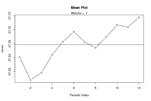
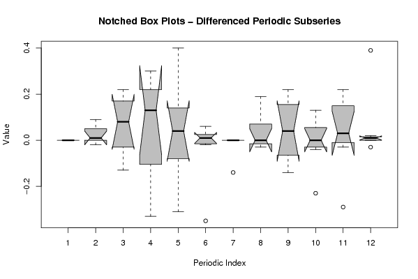
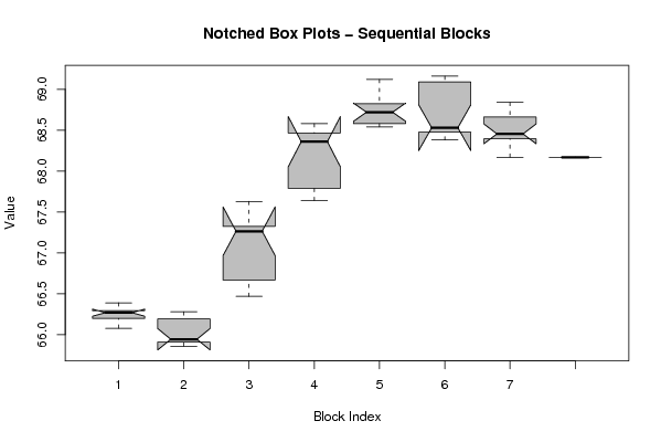
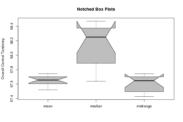
| Title produced by software | Mean Plot | ||||||||||||||||||||
| Date of computation | Tue, 16 Dec 2008 01:15:13 -0700 | ||||||||||||||||||||
| Cite this page as follows | Statistical Computations at FreeStatistics.org, Office for Research Development and Education, URL https://freestatistics.org/blog/index.php?v=date/2008/Dec/16/t1229415466nqeuks4rop8qwwr.htm/, Retrieved Wed, 15 May 2024 15:48:31 +0000 | ||||||||||||||||||||
| Statistical Computations at FreeStatistics.org, Office for Research Development and Education, URL https://freestatistics.org/blog/index.php?pk=33872, Retrieved Wed, 15 May 2024 15:48:31 +0000 | |||||||||||||||||||||
| QR Codes: | |||||||||||||||||||||
|
| |||||||||||||||||||||
| Original text written by user: | |||||||||||||||||||||
| IsPrivate? | No (this computation is public) | ||||||||||||||||||||
| User-defined keywords | |||||||||||||||||||||
| Estimated Impact | 209 | ||||||||||||||||||||
Tree of Dependent Computations | |||||||||||||||||||||
| Family? (F = Feedback message, R = changed R code, M = changed R Module, P = changed Parameters, D = changed Data) | |||||||||||||||||||||
| - [Mean Plot] [] [2008-12-16 08:15:13] [0ebe94bd950a0b1969e8ed777006e521] [Current] - D [Mean Plot] [Maxime Jonckheere...] [2009-05-13 18:45:10] [74be16979710d4c4e7c6647856088456] | |||||||||||||||||||||
| Feedback Forum | |||||||||||||||||||||
Post a new message | |||||||||||||||||||||
Dataset | |||||||||||||||||||||
| Dataseries X: | |||||||||||||||||||||
66,2 66,2 66,2 66,08 66,31 66,39 66,37 66,23 66,27 66,27 66,27 66,28 66,28 66,28 66,26 66,13 65,86 65,9 65,94 65,94 65,91 65,95 65,91 66,08 66,47 66,47 66,56 66,78 67,08 67,28 67,27 67,27 67,26 67,37 67,5 67,63 67,64 67,64 67,71 67,87 67,93 68,33 68,39 68,39 68,58 68,44 68,49 68,52 68,54 68,54 68,54 68,62 68,75 68,71 68,72 68,72 68,72 68,92 68,9 69,12 69,09 69,09 69,1 69,16 68,83 68,52 68,53 68,53 68,51 68,38 68,44 68,41 68,42 68,42 68,45 68,63 68,84 68,72 68,37 68,37 68,47 68,69 68,46 68,17 68,17 | |||||||||||||||||||||
Tables (Output of Computation) | |||||||||||||||||||||
| |||||||||||||||||||||
Figures (Output of Computation) | |||||||||||||||||||||
Input Parameters & R Code | |||||||||||||||||||||
| Parameters (Session): | |||||||||||||||||||||
| par1 = 12 ; | |||||||||||||||||||||
| Parameters (R input): | |||||||||||||||||||||
| par1 = 12 ; | |||||||||||||||||||||
| R code (references can be found in the software module): | |||||||||||||||||||||
par1 <- as.numeric(par1) | |||||||||||||||||||||