Free Statistics
of Irreproducible Research!
Description of Statistical Computation | |||||||||||||||||||||
|---|---|---|---|---|---|---|---|---|---|---|---|---|---|---|---|---|---|---|---|---|---|
| Author's title | |||||||||||||||||||||
| Author | *Unverified author* | ||||||||||||||||||||
| R Software Module | rwasp_meanplot.wasp | ||||||||||||||||||||
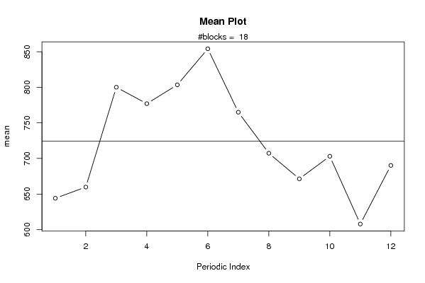
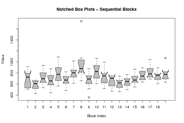
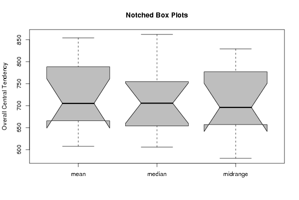
| Title produced by software | Mean Plot | ||||||||||||||||||||
| Date of computation | Mon, 15 Dec 2008 04:28:21 -0700 | ||||||||||||||||||||
| Cite this page as follows | Statistical Computations at FreeStatistics.org, Office for Research Development and Education, URL https://freestatistics.org/blog/index.php?v=date/2008/Dec/15/t12293405398id9n3w8e5emfx5.htm/, Retrieved Wed, 15 May 2024 20:56:00 +0000 | ||||||||||||||||||||
| Statistical Computations at FreeStatistics.org, Office for Research Development and Education, URL https://freestatistics.org/blog/index.php?pk=33675, Retrieved Wed, 15 May 2024 20:56:00 +0000 | |||||||||||||||||||||
| QR Codes: | |||||||||||||||||||||
|
| |||||||||||||||||||||
| Original text written by user: | |||||||||||||||||||||
| IsPrivate? | No (this computation is public) | ||||||||||||||||||||
| User-defined keywords | |||||||||||||||||||||
| Estimated Impact | 167 | ||||||||||||||||||||
Tree of Dependent Computations | |||||||||||||||||||||
| Family? (F = Feedback message, R = changed R code, M = changed R Module, P = changed Parameters, D = changed Data) | |||||||||||||||||||||
| - [Mean Plot] [prijsonderzoek be...] [2007-12-13 15:09:30] [dbf842dffc9484d9cbe357f944e71e49] - PD [Mean Plot] [Mean Plot] [2008-12-15 11:28:21] [c8d16ef416494cf54cdcc6487855358a] [Current] | |||||||||||||||||||||
| Feedback Forum | |||||||||||||||||||||
Post a new message | |||||||||||||||||||||
Dataset | |||||||||||||||||||||
| Dataseries X: | |||||||||||||||||||||
727 817 918 786 803 756 725 523 538 587 505 521 498 550 637 622 668 669 670 499 539 593 429 622 533 655 835 686 706 869 777 739 637 597 629 940 444 496 801 659 767 876 601 697 745 655 572 628 650 677 900 780 896 1092 823 735 770 915 645 566 707 785 762 712 714 823 609 620 619 638 483 535 617 698 804 824 878 1019 974 773 734 827 804 721 659 732 839 994 828 1039 1072 803 1035 922 834 1739 359 513 699 741 793 877 750 752 675 682 583 632 606 645 980 847 941 1066 936 880 808 741 780 675 782 795 873 727 998 768 714 782 578 664 560 516 752 597 716 691 752 718 737 621 472 719 497 536 653 605 637 743 719 653 675 590 527 534 463 542 568 501 678 774 665 742 715 638 656 606 498 587 677 547 871 731 752 862 619 700 667 667 650 547 637 655 703 886 896 831 741 833 750 779 655 739 845 795 1021 726 1045 915 852 772 729 755 691 729 702 702 894 765 753 876 781 776 606 775 663 649 821 771 635 1070 693 779 | |||||||||||||||||||||
Tables (Output of Computation) | |||||||||||||||||||||
| |||||||||||||||||||||
Figures (Output of Computation) | |||||||||||||||||||||
Input Parameters & R Code | |||||||||||||||||||||
| Parameters (Session): | |||||||||||||||||||||
| Parameters (R input): | |||||||||||||||||||||
| par1 = 12 ; | |||||||||||||||||||||
| R code (references can be found in the software module): | |||||||||||||||||||||
par1 <- as.numeric(par1) | |||||||||||||||||||||