Free Statistics
of Irreproducible Research!
Description of Statistical Computation | |||||||||||||||||||||||||||||||||||||||||||||
|---|---|---|---|---|---|---|---|---|---|---|---|---|---|---|---|---|---|---|---|---|---|---|---|---|---|---|---|---|---|---|---|---|---|---|---|---|---|---|---|---|---|---|---|---|---|
| Author's title | |||||||||||||||||||||||||||||||||||||||||||||
| Author | *The author of this computation has been verified* | ||||||||||||||||||||||||||||||||||||||||||||
| R Software Module | rwasp_bidensity.wasp | ||||||||||||||||||||||||||||||||||||||||||||
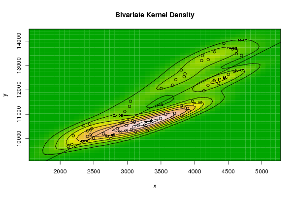
| Title produced by software | Bivariate Kernel Density Estimation | ||||||||||||||||||||||||||||||||||||||||||||
| Date of computation | Mon, 15 Dec 2008 04:02:28 -0700 | ||||||||||||||||||||||||||||||||||||||||||||
| Cite this page as follows | Statistical Computations at FreeStatistics.org, Office for Research Development and Education, URL https://freestatistics.org/blog/index.php?v=date/2008/Dec/15/t1229339081g9urmqo81ipfl56.htm/, Retrieved Wed, 15 May 2024 10:29:58 +0000 | ||||||||||||||||||||||||||||||||||||||||||||
| Statistical Computations at FreeStatistics.org, Office for Research Development and Education, URL https://freestatistics.org/blog/index.php?pk=33662, Retrieved Wed, 15 May 2024 10:29:58 +0000 | |||||||||||||||||||||||||||||||||||||||||||||
| QR Codes: | |||||||||||||||||||||||||||||||||||||||||||||
|
| |||||||||||||||||||||||||||||||||||||||||||||
| Original text written by user: | |||||||||||||||||||||||||||||||||||||||||||||
| IsPrivate? | No (this computation is public) | ||||||||||||||||||||||||||||||||||||||||||||
| User-defined keywords | |||||||||||||||||||||||||||||||||||||||||||||
| Estimated Impact | 183 | ||||||||||||||||||||||||||||||||||||||||||||
Tree of Dependent Computations | |||||||||||||||||||||||||||||||||||||||||||||
| Family? (F = Feedback message, R = changed R code, M = changed R Module, P = changed Parameters, D = changed Data) | |||||||||||||||||||||||||||||||||||||||||||||
| - [Bivariate Kernel Density Estimation] [Bivariate Kernel ...] [2008-12-15 11:02:28] [d592f629d96b926609f311957d74fcca] [Current] - D [Bivariate Kernel Density Estimation] [Bivariate Kernel ...] [2008-12-15 11:08:11] [b591abfa820a394aeb0c5ebd9cfa1091] - [Bivariate Kernel Density Estimation] [Bivariate Kernel ...] [2008-12-15 11:12:41] [b591abfa820a394aeb0c5ebd9cfa1091] - D [Bivariate Kernel Density Estimation] [Bivariate Kernel ...] [2008-12-17 12:39:29] [b591abfa820a394aeb0c5ebd9cfa1091] | |||||||||||||||||||||||||||||||||||||||||||||
| Feedback Forum | |||||||||||||||||||||||||||||||||||||||||||||
Post a new message | |||||||||||||||||||||||||||||||||||||||||||||
Dataset | |||||||||||||||||||||||||||||||||||||||||||||
| Dataseries X: | |||||||||||||||||||||||||||||||||||||||||||||
2120.88 2174.56 2196.72 2350.44 2440.25 2408.64 2472.81 2407.60 2454.62 2448.05 2497.84 2645.64 2756.76 2849.27 2921.44 2981.85 3080.58 3106.22 3119.31 3061.26 3097.31 3161.69 3257.16 3277.01 3295.32 3363.99 3494.17 3667.03 3813.06 3917.96 3895.51 3801.06 3570.12 3701.61 3862.27 3970.10 4138.52 4199.75 4290.89 4443.91 4502.64 4356.98 4591.27 4696.96 4621.40 4562.84 4202.52 4296.49 4435.23 4105.18 4116.68 3844.49 3720.98 3674.40 3857.62 3801.06 3504.37 3032.60 3047.03 2962.34 | |||||||||||||||||||||||||||||||||||||||||||||
| Dataseries Y: | |||||||||||||||||||||||||||||||||||||||||||||
9682.35 9762.12 10124.63 10540.05 10601.61 10323.73 10418.40 10092.96 10364.91 10152.09 10032.80 10204.59 10001.60 10411.75 10673.38 10539.51 10723.78 10682.06 10283.19 10377.18 10486.64 10545.38 10554.27 10532.54 10324.31 10695.25 10827.81 10872.48 10971.19 11145.65 11234.68 11333.88 10997.97 11036.89 11257.35 11533.59 11963.12 12185.15 12377.62 12512.89 12631.48 12268.53 12754.80 13407.75 13480.21 13673.28 13239.71 13557.69 13901.28 13200.58 13406.97 12538.12 12419.57 12193.88 12656.63 12812.48 12056.67 11322.38 11530.75 11114.08 | |||||||||||||||||||||||||||||||||||||||||||||
Tables (Output of Computation) | |||||||||||||||||||||||||||||||||||||||||||||
| |||||||||||||||||||||||||||||||||||||||||||||
Figures (Output of Computation) | |||||||||||||||||||||||||||||||||||||||||||||
Input Parameters & R Code | |||||||||||||||||||||||||||||||||||||||||||||
| Parameters (Session): | |||||||||||||||||||||||||||||||||||||||||||||
| par1 = 50 ; par2 = 50 ; par3 = 0 ; par4 = 0 ; par5 = 0 ; par6 = Y ; par7 = Y ; | |||||||||||||||||||||||||||||||||||||||||||||
| Parameters (R input): | |||||||||||||||||||||||||||||||||||||||||||||
| par1 = 50 ; par2 = 50 ; par3 = 0 ; par4 = 0 ; par5 = 0 ; par6 = Y ; par7 = Y ; | |||||||||||||||||||||||||||||||||||||||||||||
| R code (references can be found in the software module): | |||||||||||||||||||||||||||||||||||||||||||||
par1 <- as(par1,'numeric') | |||||||||||||||||||||||||||||||||||||||||||||