Free Statistics
of Irreproducible Research!
Description of Statistical Computation | |||||||||||||||||||||
|---|---|---|---|---|---|---|---|---|---|---|---|---|---|---|---|---|---|---|---|---|---|
| Author's title | |||||||||||||||||||||
| Author | *The author of this computation has been verified* | ||||||||||||||||||||
| R Software Module | rwasp_meanplot.wasp | ||||||||||||||||||||
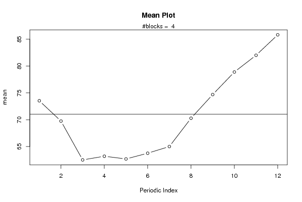
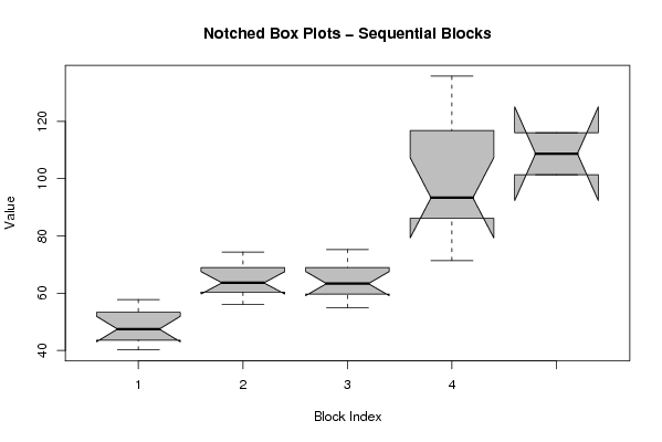
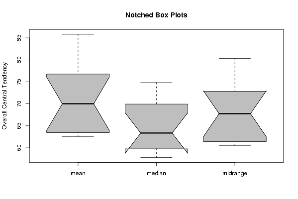
| Title produced by software | Mean Plot | ||||||||||||||||||||
| Date of computation | Mon, 15 Dec 2008 03:38:30 -0700 | ||||||||||||||||||||
| Cite this page as follows | Statistical Computations at FreeStatistics.org, Office for Research Development and Education, URL https://freestatistics.org/blog/index.php?v=date/2008/Dec/15/t1229337606jnn20ff4lpnx371.htm/, Retrieved Wed, 15 May 2024 21:01:03 +0000 | ||||||||||||||||||||
| Statistical Computations at FreeStatistics.org, Office for Research Development and Education, URL https://freestatistics.org/blog/index.php?pk=33654, Retrieved Wed, 15 May 2024 21:01:03 +0000 | |||||||||||||||||||||
| QR Codes: | |||||||||||||||||||||
|
| |||||||||||||||||||||
| Original text written by user: | |||||||||||||||||||||
| IsPrivate? | No (this computation is public) | ||||||||||||||||||||
| User-defined keywords | |||||||||||||||||||||
| Estimated Impact | 172 | ||||||||||||||||||||
Tree of Dependent Computations | |||||||||||||||||||||
| Family? (F = Feedback message, R = changed R code, M = changed R Module, P = changed Parameters, D = changed Data) | |||||||||||||||||||||
| F [Mean Plot] [workshop 3] [2007-10-26 12:14:28] [e9ffc5de6f8a7be62f22b142b5b6b1a8] F R D [Mean Plot] [Mean Plot - Bel20] [2008-11-03 18:27:03] [b591abfa820a394aeb0c5ebd9cfa1091] - D [Mean Plot] [Notched Boxplots ...] [2008-12-15 10:33:29] [adb6b6905cde49db36d59ca44433140d] - D [Mean Plot] [Notched Boxplots ...] [2008-12-15 10:38:30] [6d5cd2fe15d123a10639b4bf141c23b5] [Current] | |||||||||||||||||||||
| Feedback Forum | |||||||||||||||||||||
Post a new message | |||||||||||||||||||||
Dataset | |||||||||||||||||||||
| Dataseries X: | |||||||||||||||||||||
41.84 42.94 49.14 44.61 40.22 44.23 45.85 53.38 53.26 51.80 55.30 57.81 63.96 63.77 59.15 56.12 57.42 63.52 61.71 63.01 68.18 72.03 69.75 74.41 74.33 64.24 60.03 59.44 62.50 55.04 58.34 61.92 67.65 67.68 70.30 75.26 71.44 76.36 81.71 92.60 90.60 92.23 94.09 102.79 109.65 124.05 132.69 135.81 116.07 101.42 | |||||||||||||||||||||
Tables (Output of Computation) | |||||||||||||||||||||
| |||||||||||||||||||||
Figures (Output of Computation) | |||||||||||||||||||||
Input Parameters & R Code | |||||||||||||||||||||
| Parameters (Session): | |||||||||||||||||||||
| par1 = 12 ; | |||||||||||||||||||||
| Parameters (R input): | |||||||||||||||||||||
| par1 = 12 ; | |||||||||||||||||||||
| R code (references can be found in the software module): | |||||||||||||||||||||
par1 <- as.numeric(par1) | |||||||||||||||||||||