Free Statistics

of Irreproducible Research!

Author's title

ARIMA Forecast Totaal # niet-werkende werkzoekende mannen in het Vlaams gew...

Author

*The author of this computation has been verified*

R Software Module

rwasp_arimaforecasting.wasp

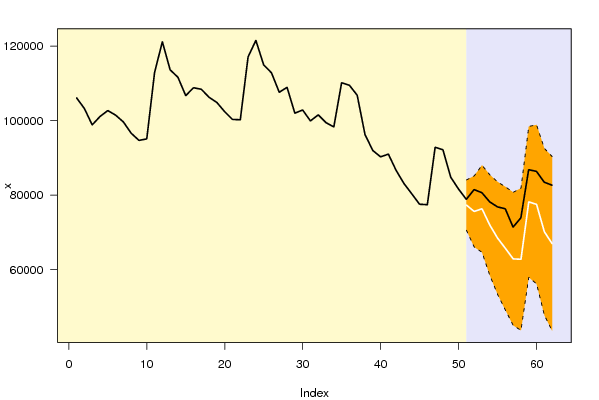
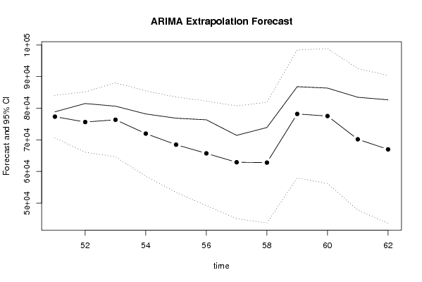
Title produced by software

ARIMA Forecasting

Date of computation

Mon, 15 Dec 2008 03:23:36 -0700

Cite this page as follows

Statistical Computations at FreeStatistics.org, Office for Research Development and Education, URL https://freestatistics.org/blog/index.php?v=date/2008/Dec/15/t1229337338xci6dvukzs3st4y.htm/, Retrieved Wed, 15 May 2024 05:53:32 +0000

Statistical Computations at FreeStatistics.org, Office for Research Development and Education, URL https://freestatistics.org/blog/index.php?pk=33650, Retrieved Wed, 15 May 2024 05:53:32 +0000

QR Codes:

Paste this QR Code to cite your computation.

Original text written by user:

IsPrivate?

No (this computation is public)

User-defined keywords

ARIMA Forecast Totaal niet-werkende werkzoekende mannen Vlaams gewest

Estimated Impact

210

Family? (F = Feedback message, R = changed R code, M = changed R Module, P = changed Parameters, D = changed Data)

F     [Univariate Data Series] [Airline data] [2007-10-18 09:58:47] [42daae401fd3def69a25014f2252b4c2]
F RMPD  [Standard Deviation-Mean Plot] [vraag 5] [2008-11-29 13:37:39] [c45c87b96bbf32ffc2144fc37d767b2e]
- RMPD    [(Partial) Autocorrelation Function] [ACF] [2008-12-12 14:04:37] [c45c87b96bbf32ffc2144fc37d767b2e]
- RMP       [ARIMA Backward Selection] [ABSM] [2008-12-12 19:09:25] [c45c87b96bbf32ffc2144fc37d767b2e]
- RMP         [ARIMA Forecasting] [] [2008-12-12 22:20:54] [a4ee3bef49b119f4bd2e925060c84f5e]
-   PD            [ARIMA Forecasting] [ARIMA Forecast To...] [2008-12-15 10:23:36] [f4b2017b314c03698059f43b95818e67] [Current]

Feedback Forum

Post a new message

Dataseries X:

Download CSV

Histogram

Boxplots

Summary of computational transaction
Raw Input	view raw input (R code)
Raw Output	view raw output of R engine
Computing time	1 seconds
R Server	'George Udny Yule' @ 72.249.76.132

\begin{tabular}{lllllllll}
\hline
Summary of computational transaction \tabularnewline
Raw Input & view raw input (R code)  \tabularnewline
Raw Output & view raw output of R engine  \tabularnewline
Computing time & 1 seconds \tabularnewline
R Server & 'George Udny Yule' @ 72.249.76.132 \tabularnewline
\hline
\end{tabular}
%Source: https://freestatistics.org/blog/index.php?pk=33650&T=0

[TABLE]
[ROW][C]Summary of computational transaction[/C][/ROW]
[ROW][C]Raw Input[/C][C]view raw input (R code) [/C][/ROW]
[ROW][C]Raw Output[/C][C]view raw output of R engine [/C][/ROW]
[ROW][C]Computing time[/C][C]1 seconds[/C][/ROW]
[ROW][C]R Server[/C][C]'George Udny Yule' @ 72.249.76.132[/C][/ROW]
[/TABLE]
Source: https://freestatistics.org/blog/index.php?pk=33650&T=0

Globally Unique Identifier (entire table): ba.freestatistics.org/blog/index.php?pk=33650&T=0

As an alternative you can also use a QR Code:

The GUIDs for individual cells are displayed in the table below:

Summary of computational transaction
Raw Input	view raw input (R code)
Raw Output	view raw output of R engine
Computing time	1 seconds
R Server	'George Udny Yule' @ 72.249.76.132

Univariate ARIMA Extrapolation Forecast
time	Y[t]	F[t]	95% LB	95% UB	p-value(H0: Y[t] = F[t])	P(F[t]>Y[t-1])	P(F[t]>Y[t-s])	P(F[t]>Y[50])
38	96279	-	-	-	-	-	-	-
39	91982	-	-	-	-	-	-	-
40	90276	-	-	-	-	-	-	-
41	90999	-	-	-	-	-	-	-
42	86622	-	-	-	-	-	-	-
43	83117	-	-	-	-	-	-	-
44	80367	-	-	-	-	-	-	-
45	77550	-	-	-	-	-	-	-
46	77443	-	-	-	-	-	-	-
47	92844	-	-	-	-	-	-	-
48	92175	-	-	-	-	-	-	-
49	84822	-	-	-	-	-	-	-
50	81632	-	-	-	-	-	-	-
51	78872	77335	70587.4368	84082.5632	0.3276	0.106	0	0.106
52	81485	75629	66086.5046	85171.4954	0.1145	0.2527	0.0013	0.1088
53	80651	76352	64664.8776	88039.1224	0.2355	0.1947	0.007	0.1879
54	78192	71975	58479.8735	85470.1265	0.1833	0.1038	0.0167	0.0804
55	76844	68470	53381.9899	83558.0101	0.1383	0.1033	0.0285	0.0437
56	76335	65720	49191.913	82248.087	0.1041	0.0936	0.0412	0.0296
57	71415	62903	45050.6257	80755.3743	0.175	0.0701	0.0539	0.0199
58	73899	62796	43711.0091	81880.9909	0.1271	0.188	0.0663	0.0265
59	86822	78197	57954.3103	98439.6897	0.2018	0.6614	0.0781	0.3697
60	86371	77528	56190.3315	98865.6685	0.2083	0.1966	0.0892	0.3531
61	83469	70175	47795.8645	92554.1355	0.1221	0.078	0.0998	0.1578
62	82662	66985	43610.7553	90359.2447	0.0943	0.0835	0.1097	0.1097

\begin{tabular}{lllllllll}
\hline
Univariate ARIMA Extrapolation Forecast \tabularnewline
time & Y[t] & F[t] & 95% LB & 95% UB & p-value(H0: Y[t] = F[t]) & P(F[t]>Y[t-1]) & P(F[t]>Y[t-s]) & P(F[t]>Y[50]) \tabularnewline
38 & 96279 & - & - & - & - & - & - & - \tabularnewline
39 & 91982 & - & - & - & - & - & - & - \tabularnewline
40 & 90276 & - & - & - & - & - & - & - \tabularnewline
41 & 90999 & - & - & - & - & - & - & - \tabularnewline
42 & 86622 & - & - & - & - & - & - & - \tabularnewline
43 & 83117 & - & - & - & - & - & - & - \tabularnewline
44 & 80367 & - & - & - & - & - & - & - \tabularnewline
45 & 77550 & - & - & - & - & - & - & - \tabularnewline
46 & 77443 & - & - & - & - & - & - & - \tabularnewline
47 & 92844 & - & - & - & - & - & - & - \tabularnewline
48 & 92175 & - & - & - & - & - & - & - \tabularnewline
49 & 84822 & - & - & - & - & - & - & - \tabularnewline
50 & 81632 & - & - & - & - & - & - & - \tabularnewline
51 & 78872 & 77335 & 70587.4368 & 84082.5632 & 0.3276 & 0.106 & 0 & 0.106 \tabularnewline
52 & 81485 & 75629 & 66086.5046 & 85171.4954 & 0.1145 & 0.2527 & 0.0013 & 0.1088 \tabularnewline
53 & 80651 & 76352 & 64664.8776 & 88039.1224 & 0.2355 & 0.1947 & 0.007 & 0.1879 \tabularnewline
54 & 78192 & 71975 & 58479.8735 & 85470.1265 & 0.1833 & 0.1038 & 0.0167 & 0.0804 \tabularnewline
55 & 76844 & 68470 & 53381.9899 & 83558.0101 & 0.1383 & 0.1033 & 0.0285 & 0.0437 \tabularnewline
56 & 76335 & 65720 & 49191.913 & 82248.087 & 0.1041 & 0.0936 & 0.0412 & 0.0296 \tabularnewline
57 & 71415 & 62903 & 45050.6257 & 80755.3743 & 0.175 & 0.0701 & 0.0539 & 0.0199 \tabularnewline
58 & 73899 & 62796 & 43711.0091 & 81880.9909 & 0.1271 & 0.188 & 0.0663 & 0.0265 \tabularnewline
59 & 86822 & 78197 & 57954.3103 & 98439.6897 & 0.2018 & 0.6614 & 0.0781 & 0.3697 \tabularnewline
60 & 86371 & 77528 & 56190.3315 & 98865.6685 & 0.2083 & 0.1966 & 0.0892 & 0.3531 \tabularnewline
61 & 83469 & 70175 & 47795.8645 & 92554.1355 & 0.1221 & 0.078 & 0.0998 & 0.1578 \tabularnewline
62 & 82662 & 66985 & 43610.7553 & 90359.2447 & 0.0943 & 0.0835 & 0.1097 & 0.1097 \tabularnewline
\hline
\end{tabular}
%Source: https://freestatistics.org/blog/index.php?pk=33650&T=1

[TABLE]
[ROW][C]Univariate ARIMA Extrapolation Forecast[/C][/ROW]
[ROW][C]time[/C][C]Y[t][/C][C]F[t][/C][C]95% LB[/C][C]95% UB[/C][C]p-value(H0: Y[t] = F[t])[/C][C]P(F[t]>Y[t-1])[/C][C]P(F[t]>Y[t-s])[/C][C]P(F[t]>Y[50])[/C][/ROW]
[ROW][C]38[/C][C]96279[/C][C]-[/C][C]-[/C][C]-[/C][C]-[/C][C]-[/C][C]-[/C][C]-[/C][/ROW]
[ROW][C]39[/C][C]91982[/C][C]-[/C][C]-[/C][C]-[/C][C]-[/C][C]-[/C][C]-[/C][C]-[/C][/ROW]
[ROW][C]40[/C][C]90276[/C][C]-[/C][C]-[/C][C]-[/C][C]-[/C][C]-[/C][C]-[/C][C]-[/C][/ROW]
[ROW][C]41[/C][C]90999[/C][C]-[/C][C]-[/C][C]-[/C][C]-[/C][C]-[/C][C]-[/C][C]-[/C][/ROW]
[ROW][C]42[/C][C]86622[/C][C]-[/C][C]-[/C][C]-[/C][C]-[/C][C]-[/C][C]-[/C][C]-[/C][/ROW]
[ROW][C]43[/C][C]83117[/C][C]-[/C][C]-[/C][C]-[/C][C]-[/C][C]-[/C][C]-[/C][C]-[/C][/ROW]
[ROW][C]44[/C][C]80367[/C][C]-[/C][C]-[/C][C]-[/C][C]-[/C][C]-[/C][C]-[/C][C]-[/C][/ROW]
[ROW][C]45[/C][C]77550[/C][C]-[/C][C]-[/C][C]-[/C][C]-[/C][C]-[/C][C]-[/C][C]-[/C][/ROW]
[ROW][C]46[/C][C]77443[/C][C]-[/C][C]-[/C][C]-[/C][C]-[/C][C]-[/C][C]-[/C][C]-[/C][/ROW]
[ROW][C]47[/C][C]92844[/C][C]-[/C][C]-[/C][C]-[/C][C]-[/C][C]-[/C][C]-[/C][C]-[/C][/ROW]
[ROW][C]48[/C][C]92175[/C][C]-[/C][C]-[/C][C]-[/C][C]-[/C][C]-[/C][C]-[/C][C]-[/C][/ROW]
[ROW][C]49[/C][C]84822[/C][C]-[/C][C]-[/C][C]-[/C][C]-[/C][C]-[/C][C]-[/C][C]-[/C][/ROW]
[ROW][C]50[/C][C]81632[/C][C]-[/C][C]-[/C][C]-[/C][C]-[/C][C]-[/C][C]-[/C][C]-[/C][/ROW]
[ROW][C]51[/C][C]78872[/C][C]77335[/C][C]70587.4368[/C][C]84082.5632[/C][C]0.3276[/C][C]0.106[/C][C]0[/C][C]0.106[/C][/ROW]
[ROW][C]52[/C][C]81485[/C][C]75629[/C][C]66086.5046[/C][C]85171.4954[/C][C]0.1145[/C][C]0.2527[/C][C]0.0013[/C][C]0.1088[/C][/ROW]
[ROW][C]53[/C][C]80651[/C][C]76352[/C][C]64664.8776[/C][C]88039.1224[/C][C]0.2355[/C][C]0.1947[/C][C]0.007[/C][C]0.1879[/C][/ROW]
[ROW][C]54[/C][C]78192[/C][C]71975[/C][C]58479.8735[/C][C]85470.1265[/C][C]0.1833[/C][C]0.1038[/C][C]0.0167[/C][C]0.0804[/C][/ROW]
[ROW][C]55[/C][C]76844[/C][C]68470[/C][C]53381.9899[/C][C]83558.0101[/C][C]0.1383[/C][C]0.1033[/C][C]0.0285[/C][C]0.0437[/C][/ROW]
[ROW][C]56[/C][C]76335[/C][C]65720[/C][C]49191.913[/C][C]82248.087[/C][C]0.1041[/C][C]0.0936[/C][C]0.0412[/C][C]0.0296[/C][/ROW]
[ROW][C]57[/C][C]71415[/C][C]62903[/C][C]45050.6257[/C][C]80755.3743[/C][C]0.175[/C][C]0.0701[/C][C]0.0539[/C][C]0.0199[/C][/ROW]
[ROW][C]58[/C][C]73899[/C][C]62796[/C][C]43711.0091[/C][C]81880.9909[/C][C]0.1271[/C][C]0.188[/C][C]0.0663[/C][C]0.0265[/C][/ROW]
[ROW][C]59[/C][C]86822[/C][C]78197[/C][C]57954.3103[/C][C]98439.6897[/C][C]0.2018[/C][C]0.6614[/C][C]0.0781[/C][C]0.3697[/C][/ROW]
[ROW][C]60[/C][C]86371[/C][C]77528[/C][C]56190.3315[/C][C]98865.6685[/C][C]0.2083[/C][C]0.1966[/C][C]0.0892[/C][C]0.3531[/C][/ROW]
[ROW][C]61[/C][C]83469[/C][C]70175[/C][C]47795.8645[/C][C]92554.1355[/C][C]0.1221[/C][C]0.078[/C][C]0.0998[/C][C]0.1578[/C][/ROW]
[ROW][C]62[/C][C]82662[/C][C]66985[/C][C]43610.7553[/C][C]90359.2447[/C][C]0.0943[/C][C]0.0835[/C][C]0.1097[/C][C]0.1097[/C][/ROW]
[/TABLE]
Source: https://freestatistics.org/blog/index.php?pk=33650&T=1

Globally Unique Identifier (entire table): ba.freestatistics.org/blog/index.php?pk=33650&T=1

As an alternative you can also use a QR Code:

The GUIDs for individual cells are displayed in the table below:

Univariate ARIMA Extrapolation Forecast
time	Y[t]	F[t]	95% LB	95% UB	p-value(H0: Y[t] = F[t])	P(F[t]>Y[t-1])	P(F[t]>Y[t-s])	P(F[t]>Y[50])
38	96279	-	-	-	-	-	-	-
39	91982	-	-	-	-	-	-	-
40	90276	-	-	-	-	-	-	-
41	90999	-	-	-	-	-	-	-
42	86622	-	-	-	-	-	-	-
43	83117	-	-	-	-	-	-	-
44	80367	-	-	-	-	-	-	-
45	77550	-	-	-	-	-	-	-
46	77443	-	-	-	-	-	-	-
47	92844	-	-	-	-	-	-	-
48	92175	-	-	-	-	-	-	-
49	84822	-	-	-	-	-	-	-
50	81632	-	-	-	-	-	-	-
51	78872	77335	70587.4368	84082.5632	0.3276	0.106	0	0.106
52	81485	75629	66086.5046	85171.4954	0.1145	0.2527	0.0013	0.1088
53	80651	76352	64664.8776	88039.1224	0.2355	0.1947	0.007	0.1879
54	78192	71975	58479.8735	85470.1265	0.1833	0.1038	0.0167	0.0804
55	76844	68470	53381.9899	83558.0101	0.1383	0.1033	0.0285	0.0437
56	76335	65720	49191.913	82248.087	0.1041	0.0936	0.0412	0.0296
57	71415	62903	45050.6257	80755.3743	0.175	0.0701	0.0539	0.0199
58	73899	62796	43711.0091	81880.9909	0.1271	0.188	0.0663	0.0265
59	86822	78197	57954.3103	98439.6897	0.2018	0.6614	0.0781	0.3697
60	86371	77528	56190.3315	98865.6685	0.2083	0.1966	0.0892	0.3531
61	83469	70175	47795.8645	92554.1355	0.1221	0.078	0.0998	0.1578
62	82662	66985	43610.7553	90359.2447	0.0943	0.0835	0.1097	0.1097

Univariate ARIMA Extrapolation Forecast Performance
time	% S.E.	PE	MAPE	Sq.E	MSE	RMSE
51	0.0445	0.0199	0.0017	2362369	196864.0833	443.6937
52	0.0644	0.0774	0.0065	34292736	2857728	1690.4816
53	0.0781	0.0563	0.0047	18481401	1540116.75	1241.0144
54	0.0957	0.0864	0.0072	38651089	3220924.0833	1794.6933
55	0.1124	0.1223	0.0102	70123876	5843656.3333	2417.3656
56	0.1283	0.1615	0.0135	112678225	9389852.0833	3064.2866
57	0.1448	0.1353	0.0113	72454144	6037845.3333	2457.2027
58	0.1551	0.1768	0.0147	123276609	10273050.75	3205.16
59	0.1321	0.1103	0.0092	74390625	6199218.75	2489.823
60	0.1404	0.1141	0.0095	78198649	6516554.0833	2552.7542
61	0.1627	0.1894	0.0158	176730436	14727536.3333	3837.6472
62	0.178	0.234	0.0195	245768329	20480694.0833	4525.5601

\begin{tabular}{lllllllll}
\hline
Univariate ARIMA Extrapolation Forecast Performance \tabularnewline
time & % S.E. & PE & MAPE & Sq.E & MSE & RMSE \tabularnewline
51 & 0.0445 & 0.0199 & 0.0017 & 2362369 & 196864.0833 & 443.6937 \tabularnewline
52 & 0.0644 & 0.0774 & 0.0065 & 34292736 & 2857728 & 1690.4816 \tabularnewline
53 & 0.0781 & 0.0563 & 0.0047 & 18481401 & 1540116.75 & 1241.0144 \tabularnewline
54 & 0.0957 & 0.0864 & 0.0072 & 38651089 & 3220924.0833 & 1794.6933 \tabularnewline
55 & 0.1124 & 0.1223 & 0.0102 & 70123876 & 5843656.3333 & 2417.3656 \tabularnewline
56 & 0.1283 & 0.1615 & 0.0135 & 112678225 & 9389852.0833 & 3064.2866 \tabularnewline
57 & 0.1448 & 0.1353 & 0.0113 & 72454144 & 6037845.3333 & 2457.2027 \tabularnewline
58 & 0.1551 & 0.1768 & 0.0147 & 123276609 & 10273050.75 & 3205.16 \tabularnewline
59 & 0.1321 & 0.1103 & 0.0092 & 74390625 & 6199218.75 & 2489.823 \tabularnewline
60 & 0.1404 & 0.1141 & 0.0095 & 78198649 & 6516554.0833 & 2552.7542 \tabularnewline
61 & 0.1627 & 0.1894 & 0.0158 & 176730436 & 14727536.3333 & 3837.6472 \tabularnewline
62 & 0.178 & 0.234 & 0.0195 & 245768329 & 20480694.0833 & 4525.5601 \tabularnewline
\hline
\end{tabular}
%Source: https://freestatistics.org/blog/index.php?pk=33650&T=2

[TABLE]
[ROW][C]Univariate ARIMA Extrapolation Forecast Performance[/C][/ROW]
[ROW][C]time[/C][C]% S.E.[/C][C]PE[/C][C]MAPE[/C][C]Sq.E[/C][C]MSE[/C][C]RMSE[/C][/ROW]
[ROW][C]51[/C][C]0.0445[/C][C]0.0199[/C][C]0.0017[/C][C]2362369[/C][C]196864.0833[/C][C]443.6937[/C][/ROW]
[ROW][C]52[/C][C]0.0644[/C][C]0.0774[/C][C]0.0065[/C][C]34292736[/C][C]2857728[/C][C]1690.4816[/C][/ROW]
[ROW][C]53[/C][C]0.0781[/C][C]0.0563[/C][C]0.0047[/C][C]18481401[/C][C]1540116.75[/C][C]1241.0144[/C][/ROW]
[ROW][C]54[/C][C]0.0957[/C][C]0.0864[/C][C]0.0072[/C][C]38651089[/C][C]3220924.0833[/C][C]1794.6933[/C][/ROW]
[ROW][C]55[/C][C]0.1124[/C][C]0.1223[/C][C]0.0102[/C][C]70123876[/C][C]5843656.3333[/C][C]2417.3656[/C][/ROW]
[ROW][C]56[/C][C]0.1283[/C][C]0.1615[/C][C]0.0135[/C][C]112678225[/C][C]9389852.0833[/C][C]3064.2866[/C][/ROW]
[ROW][C]57[/C][C]0.1448[/C][C]0.1353[/C][C]0.0113[/C][C]72454144[/C][C]6037845.3333[/C][C]2457.2027[/C][/ROW]
[ROW][C]58[/C][C]0.1551[/C][C]0.1768[/C][C]0.0147[/C][C]123276609[/C][C]10273050.75[/C][C]3205.16[/C][/ROW]
[ROW][C]59[/C][C]0.1321[/C][C]0.1103[/C][C]0.0092[/C][C]74390625[/C][C]6199218.75[/C][C]2489.823[/C][/ROW]
[ROW][C]60[/C][C]0.1404[/C][C]0.1141[/C][C]0.0095[/C][C]78198649[/C][C]6516554.0833[/C][C]2552.7542[/C][/ROW]
[ROW][C]61[/C][C]0.1627[/C][C]0.1894[/C][C]0.0158[/C][C]176730436[/C][C]14727536.3333[/C][C]3837.6472[/C][/ROW]
[ROW][C]62[/C][C]0.178[/C][C]0.234[/C][C]0.0195[/C][C]245768329[/C][C]20480694.0833[/C][C]4525.5601[/C][/ROW]
[/TABLE]
Source: https://freestatistics.org/blog/index.php?pk=33650&T=2

Globally Unique Identifier (entire table): ba.freestatistics.org/blog/index.php?pk=33650&T=2

As an alternative you can also use a QR Code:

The GUIDs for individual cells are displayed in the table below:

Univariate ARIMA Extrapolation Forecast Performance
time	% S.E.	PE	MAPE	Sq.E	MSE	RMSE
51	0.0445	0.0199	0.0017	2362369	196864.0833	443.6937
52	0.0644	0.0774	0.0065	34292736	2857728	1690.4816
53	0.0781	0.0563	0.0047	18481401	1540116.75	1241.0144
54	0.0957	0.0864	0.0072	38651089	3220924.0833	1794.6933
55	0.1124	0.1223	0.0102	70123876	5843656.3333	2417.3656
56	0.1283	0.1615	0.0135	112678225	9389852.0833	3064.2866
57	0.1448	0.1353	0.0113	72454144	6037845.3333	2457.2027
58	0.1551	0.1768	0.0147	123276609	10273050.75	3205.16
59	0.1321	0.1103	0.0092	74390625	6199218.75	2489.823
60	0.1404	0.1141	0.0095	78198649	6516554.0833	2552.7542
61	0.1627	0.1894	0.0158	176730436	14727536.3333	3837.6472
62	0.178	0.234	0.0195	245768329	20480694.0833	4525.5601

Figure 1

PNG link

Postscript link

PDF link

Figure 2

PNG link

Postscript link

PDF link

Parameters (Session):

par1 = 12 ; par2 = 1 ; par3 = 1 ; par4 = 1 ; par5 = 12 ; par6 = 0 ; par7 = 0 ; par8 = 0 ; par9 = 0 ; par10 = FALSE ;

Parameters (R input):

par1 = 12 ; par2 = 1 ; par3 = 1 ; par4 = 1 ; par5 = 12 ; par6 = 0 ; par7 = 0 ; par8 = 0 ; par9 = 0 ; par10 = FALSE ;

R code (references can be found in the software module):

par1 <- as.numeric(par1) #cut off periods
par2 <- as.numeric(par2) #lambda
par3 <- as.numeric(par3) #degree of non-seasonal differencing
par4 <- as.numeric(par4) #degree of seasonal differencing
par5 <- as.numeric(par5) #seasonal period
par6 <- as.numeric(par6) #p
par7 <- as.numeric(par7) #q
par8 <- as.numeric(par8) #P
par9 <- as.numeric(par9) #Q
if (par10 == 'TRUE') par10 <- TRUE
if (par10 == 'FALSE') par10 <- FALSE
if (par2 == 0) x <- log(x)
if (par2 != 0) x <- x^par2
lx <- length(x)
first <- lx - 2*par1
nx <- lx - par1
nx1 <- nx + 1
fx <- lx - nx
if (fx < 1) {
fx <- par5
nx1 <- lx + fx - 1
first <- lx - 2*fx
}
first <- 1
if (fx < 3) fx <- round(lx/10,0)
(arima.out <- arima(x[1:nx], order=c(par6,par3,par7), seasonal=list(order=c(par8,par4,par9), period=par5), include.mean=par10, method='ML'))
(forecast <- predict(arima.out,fx))
(lb <- forecast$pred - 1.96 * forecast$se)
(ub <- forecast$pred + 1.96 * forecast$se)
if (par2 == 0) {
x <- exp(x)
forecast$pred <- exp(forecast$pred)
lb <- exp(lb)
ub <- exp(ub)
}
if (par2 != 0) {
x <- x^(1/par2)
forecast$pred <- forecast$pred^(1/par2)
lb <- lb^(1/par2)
ub <- ub^(1/par2)
}
if (par2 < 0) {
olb <- lb
lb <- ub
ub <- olb
}
(actandfor <- c(x[1:nx], forecast$pred))
(perc.se <- (ub-forecast$pred)/1.96/forecast$pred)
bitmap(file='test1.png')
opar <- par(mar=c(4,4,2,2),las=1)
ylim <- c( min(x[first:nx],lb), max(x[first:nx],ub))
plot(x,ylim=ylim,type='n',xlim=c(first,lx))
usr <- par('usr')
rect(usr[1],usr[3],nx+1,usr[4],border=NA,col='lemonchiffon')
rect(nx1,usr[3],usr[2],usr[4],border=NA,col='lavender')
abline(h= (-3:3)*2 , col ='gray', lty =3)
polygon( c(nx1:lx,lx:nx1), c(lb,rev(ub)), col = 'orange', lty=2,border=NA)
lines(nx1:lx, lb , lty=2)
lines(nx1:lx, ub , lty=2)
lines(x, lwd=2)
lines(nx1:lx, forecast$pred , lwd=2 , col ='white')
box()
par(opar)
dev.off()
prob.dec <- array(NA, dim=fx)
prob.sdec <- array(NA, dim=fx)
prob.ldec <- array(NA, dim=fx)
prob.pval <- array(NA, dim=fx)
perf.pe <- array(0, dim=fx)
perf.mape <- array(0, dim=fx)
perf.se <- array(0, dim=fx)
perf.mse <- array(0, dim=fx)
perf.rmse <- array(0, dim=fx)
for (i in 1:fx) {
locSD <- (ub[i] - forecast$pred[i]) / 1.96
perf.pe[i] = (x[nx+i] - forecast$pred[i]) / forecast$pred[i]
perf.mape[i] = perf.mape[i] + abs(perf.pe[i])
perf.se[i] = (x[nx+i] - forecast$pred[i])^2
perf.mse[i] = perf.mse[i] + perf.se[i]
prob.dec[i] = pnorm((x[nx+i-1] - forecast$pred[i]) / locSD)
prob.sdec[i] = pnorm((x[nx+i-par5] - forecast$pred[i]) / locSD)
prob.ldec[i] = pnorm((x[nx] - forecast$pred[i]) / locSD)
prob.pval[i] = pnorm(abs(x[nx+i] - forecast$pred[i]) / locSD)
}
perf.mape = perf.mape / fx
perf.mse = perf.mse / fx
perf.rmse = sqrt(perf.mse)
bitmap(file='test2.png')
plot(forecast$pred, pch=19, type='b',main='ARIMA Extrapolation Forecast', ylab='Forecast and 95% CI', xlab='time',ylim=c(min(lb),max(ub)))
dum <- forecast$pred
dum[1:12] <- x[(nx+1):lx]
lines(dum, lty=1)
lines(ub,lty=3)
lines(lb,lty=3)
dev.off()
load(file='createtable')
a<-table.start()
a<-table.row.start(a)
a<-table.element(a,'Univariate ARIMA Extrapolation Forecast',9,TRUE)
a<-table.row.end(a)
a<-table.row.start(a)
a<-table.element(a,'time',1,header=TRUE)
a<-table.element(a,'Y[t]',1,header=TRUE)
a<-table.element(a,'F[t]',1,header=TRUE)
a<-table.element(a,'95% LB',1,header=TRUE)
a<-table.element(a,'95% UB',1,header=TRUE)
a<-table.element(a,'p-value
(H0: Y[t] = F[t])',1,header=TRUE)
a<-table.element(a,'P(F[t]>Y[t-1])',1,header=TRUE)
a<-table.element(a,'P(F[t]>Y[t-s])',1,header=TRUE)
mylab <- paste('P(F[t]>Y[',nx,sep='')
mylab <- paste(mylab,'])',sep='')
a<-table.element(a,mylab,1,header=TRUE)
a<-table.row.end(a)
for (i in (nx-par5):nx) {
a<-table.row.start(a)
a<-table.element(a,i,header=TRUE)
a<-table.element(a,x[i])
a<-table.element(a,'-')
a<-table.element(a,'-')
a<-table.element(a,'-')
a<-table.element(a,'-')
a<-table.element(a,'-')
a<-table.element(a,'-')
a<-table.element(a,'-')
a<-table.row.end(a)
}
for (i in 1:fx) {
a<-table.row.start(a)
a<-table.element(a,nx+i,header=TRUE)
a<-table.element(a,round(x[nx+i],4))
a<-table.element(a,round(forecast$pred[i],4))
a<-table.element(a,round(lb[i],4))
a<-table.element(a,round(ub[i],4))
a<-table.element(a,round((1-prob.pval[i]),4))
a<-table.element(a,round((1-prob.dec[i]),4))
a<-table.element(a,round((1-prob.sdec[i]),4))
a<-table.element(a,round((1-prob.ldec[i]),4))
a<-table.row.end(a)
}
a<-table.end(a)
table.save(a,file='mytable.tab')
a<-table.start()
a<-table.row.start(a)
a<-table.element(a,'Univariate ARIMA Extrapolation Forecast Performance',7,TRUE)
a<-table.row.end(a)
a<-table.row.start(a)
a<-table.element(a,'time',1,header=TRUE)
a<-table.element(a,'% S.E.',1,header=TRUE)
a<-table.element(a,'PE',1,header=TRUE)
a<-table.element(a,'MAPE',1,header=TRUE)
a<-table.element(a,'Sq.E',1,header=TRUE)
a<-table.element(a,'MSE',1,header=TRUE)
a<-table.element(a,'RMSE',1,header=TRUE)
a<-table.row.end(a)
for (i in 1:fx) {
a<-table.row.start(a)
a<-table.element(a,nx+i,header=TRUE)
a<-table.element(a,round(perc.se[i],4))
a<-table.element(a,round(perf.pe[i],4))
a<-table.element(a,round(perf.mape[i],4))
a<-table.element(a,round(perf.se[i],4))
a<-table.element(a,round(perf.mse[i],4))
a<-table.element(a,round(perf.rmse[i],4))
a<-table.row.end(a)
}
a<-table.end(a)
table.save(a,file='mytable1.tab')

Free Statistics

Description of Statistical Computation

ARIMA Forecast Totaal # niet-werkende werkzoekende mannen in het Vlaams gew...

Tree of Dependent Computations

Dataset

Tables (Output of Computation)

Figures (Output of Computation)

Input Parameters & R Code