Free Statistics
of Irreproducible Research!
Description of Statistical Computation | |||||||||||||||||||||||||||||||||||||||||||||||||||||||||||||
|---|---|---|---|---|---|---|---|---|---|---|---|---|---|---|---|---|---|---|---|---|---|---|---|---|---|---|---|---|---|---|---|---|---|---|---|---|---|---|---|---|---|---|---|---|---|---|---|---|---|---|---|---|---|---|---|---|---|---|---|---|---|
| Author's title | |||||||||||||||||||||||||||||||||||||||||||||||||||||||||||||
| Author | *The author of this computation has been verified* | ||||||||||||||||||||||||||||||||||||||||||||||||||||||||||||
| R Software Module | rwasp_linear_regression.wasp | ||||||||||||||||||||||||||||||||||||||||||||||||||||||||||||
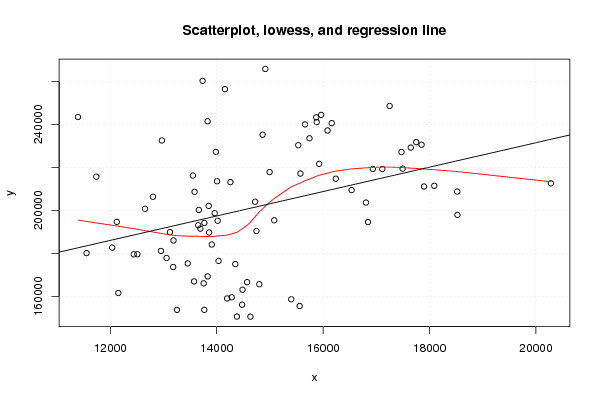
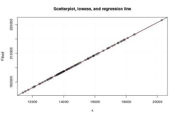
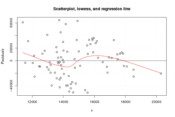
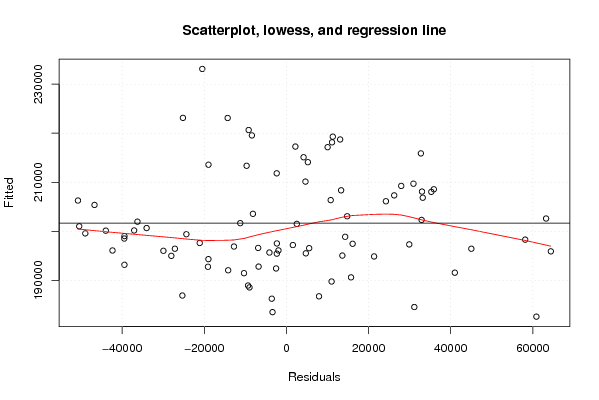
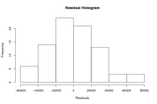
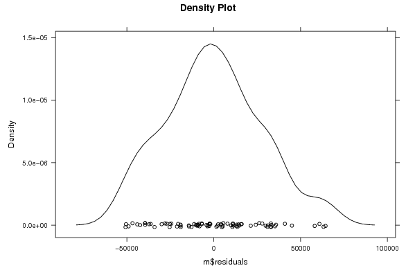
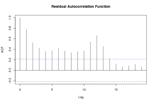
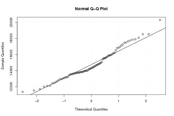
| Title produced by software | Linear Regression Graphical Model Validation | ||||||||||||||||||||||||||||||||||||||||||||||||||||||||||||
| Date of computation | Sun, 14 Dec 2008 11:25:57 -0700 | ||||||||||||||||||||||||||||||||||||||||||||||||||||||||||||
| Cite this page as follows | Statistical Computations at FreeStatistics.org, Office for Research Development and Education, URL https://freestatistics.org/blog/index.php?v=date/2008/Dec/14/t1229279477sus2dhncl7ufg0p.htm/, Retrieved Wed, 15 May 2024 16:04:25 +0000 | ||||||||||||||||||||||||||||||||||||||||||||||||||||||||||||
| Statistical Computations at FreeStatistics.org, Office for Research Development and Education, URL https://freestatistics.org/blog/index.php?pk=33527, Retrieved Wed, 15 May 2024 16:04:25 +0000 | |||||||||||||||||||||||||||||||||||||||||||||||||||||||||||||
| QR Codes: | |||||||||||||||||||||||||||||||||||||||||||||||||||||||||||||
|
| |||||||||||||||||||||||||||||||||||||||||||||||||||||||||||||
| Original text written by user: | |||||||||||||||||||||||||||||||||||||||||||||||||||||||||||||
| IsPrivate? | No (this computation is public) | ||||||||||||||||||||||||||||||||||||||||||||||||||||||||||||
| User-defined keywords | |||||||||||||||||||||||||||||||||||||||||||||||||||||||||||||
| Estimated Impact | 128 | ||||||||||||||||||||||||||||||||||||||||||||||||||||||||||||
Tree of Dependent Computations | |||||||||||||||||||||||||||||||||||||||||||||||||||||||||||||
| Family? (F = Feedback message, R = changed R code, M = changed R Module, P = changed Parameters, D = changed Data) | |||||||||||||||||||||||||||||||||||||||||||||||||||||||||||||
| - [ARIMA Backward Selection] [ARMA backward sel...] [2007-12-20 15:28:14] [74be16979710d4c4e7c6647856088456] - RMPD [ARIMA Forecasting] [forecasting] [2008-01-07 19:49:31] [74be16979710d4c4e7c6647856088456] - RMPD [Linear Regression Graphical Model Validation] [Simple Linear Reg...] [2008-12-14 18:25:57] [5925747fb2a6bb4cfcd8015825ee5e92] [Current] | |||||||||||||||||||||||||||||||||||||||||||||||||||||||||||||
| Feedback Forum | |||||||||||||||||||||||||||||||||||||||||||||||||||||||||||||
Post a new message | |||||||||||||||||||||||||||||||||||||||||||||||||||||||||||||
Dataset | |||||||||||||||||||||||||||||||||||||||||||||||||||||||||||||
| Dataseries X: | |||||||||||||||||||||||||||||||||||||||||||||||||||||||||||||
11554,5 13182,1 14800,1 12150,7 14478,2 13253,9 12036,8 12653,2 14035,4 14571,4 15400,9 14283,2 14485,3 14196,3 15559,1 13767,4 14634 14381,1 12509,9 12122,3 13122,3 13908,7 13456,5 12441,6 12953 13057,2 14350,1 13830,2 13755,5 13574,4 12802,6 11737,3 13850,2 15081,8 13653,3 14019,1 13962 13768,7 14747,1 13858,1 13188 13693,1 12970 11392,8 13985,2 14994,7 13584,7 14257,8 13553,4 14007,3 16535,8 14721,4 13664,6 16805,9 13829,4 13735,6 15870,5 15962,4 15744,1 16083,7 14863,9 15533,1 17473,1 15925,5 15573,7 17495 14155,8 14913,9 17250,4 15879,8 17647,8 17749,9 17111,8 16934,8 20280 16238,2 17896,1 18089,3 15660 16162,4 17850,1 18520,4 18524,7 16843,7 | |||||||||||||||||||||||||||||||||||||||||||||||||||||||||||||
| Dataseries Y: | |||||||||||||||||||||||||||||||||||||||||||||||||||||||||||||
180144 173666 165688 161570 156145 153730 182698 200765 176512 166618 158644 159585 163095 159044 155511 153745 150569 150605 179612 194690 189917 184128 175335 179566 181140 177876 175041 169292 166070 166972 206348 215706 202108 195411 193111 195198 198770 194163 190420 189733 186029 191531 232571 243477 227247 217859 208679 213188 216234 213586 209465 204045 200237 203666 241476 260307 243324 244460 233575 237217 235243 230354 227184 221678 217142 219452 256446 265845 248624 241114 229245 231805 219277 219313 212610 214771 211142 211457 240048 240636 230580 208795 197922 194596 | |||||||||||||||||||||||||||||||||||||||||||||||||||||||||||||
Tables (Output of Computation) | |||||||||||||||||||||||||||||||||||||||||||||||||||||||||||||
| |||||||||||||||||||||||||||||||||||||||||||||||||||||||||||||
Figures (Output of Computation) | |||||||||||||||||||||||||||||||||||||||||||||||||||||||||||||
Input Parameters & R Code | |||||||||||||||||||||||||||||||||||||||||||||||||||||||||||||
| Parameters (Session): | |||||||||||||||||||||||||||||||||||||||||||||||||||||||||||||
| par1 = 36 ; par2 = 1.3 ; par3 = 1 ; par4 = 1 ; par5 = 12 ; | |||||||||||||||||||||||||||||||||||||||||||||||||||||||||||||
| Parameters (R input): | |||||||||||||||||||||||||||||||||||||||||||||||||||||||||||||
| par1 = 0 ; | |||||||||||||||||||||||||||||||||||||||||||||||||||||||||||||
| R code (references can be found in the software module): | |||||||||||||||||||||||||||||||||||||||||||||||||||||||||||||
par1 <- as.numeric(par1) | |||||||||||||||||||||||||||||||||||||||||||||||||||||||||||||