Free Statistics
of Irreproducible Research!
Description of Statistical Computation | |||||||||||||||||||||||||||||||||||||||||||||||||||||||||||||||||||||||||||||||||
|---|---|---|---|---|---|---|---|---|---|---|---|---|---|---|---|---|---|---|---|---|---|---|---|---|---|---|---|---|---|---|---|---|---|---|---|---|---|---|---|---|---|---|---|---|---|---|---|---|---|---|---|---|---|---|---|---|---|---|---|---|---|---|---|---|---|---|---|---|---|---|---|---|---|---|---|---|---|---|---|---|---|
| Author's title | |||||||||||||||||||||||||||||||||||||||||||||||||||||||||||||||||||||||||||||||||
| Author | *The author of this computation has been verified* | ||||||||||||||||||||||||||||||||||||||||||||||||||||||||||||||||||||||||||||||||
| R Software Module | rwasp_bootstrapplot.wasp | ||||||||||||||||||||||||||||||||||||||||||||||||||||||||||||||||||||||||||||||||
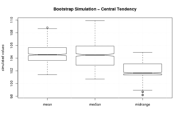
| Title produced by software | Blocked Bootstrap Plot - Central Tendency | ||||||||||||||||||||||||||||||||||||||||||||||||||||||||||||||||||||||||||||||||
| Date of computation | Sun, 14 Dec 2008 10:29:20 -0700 | ||||||||||||||||||||||||||||||||||||||||||||||||||||||||||||||||||||||||||||||||
| Cite this page as follows | Statistical Computations at FreeStatistics.org, Office for Research Development and Education, URL https://freestatistics.org/blog/index.php?v=date/2008/Dec/14/t1229275809jc5bxjm5y21kax0.htm/, Retrieved Wed, 15 May 2024 23:56:51 +0000 | ||||||||||||||||||||||||||||||||||||||||||||||||||||||||||||||||||||||||||||||||
| Statistical Computations at FreeStatistics.org, Office for Research Development and Education, URL https://freestatistics.org/blog/index.php?pk=33496, Retrieved Wed, 15 May 2024 23:56:51 +0000 | |||||||||||||||||||||||||||||||||||||||||||||||||||||||||||||||||||||||||||||||||
| QR Codes: | |||||||||||||||||||||||||||||||||||||||||||||||||||||||||||||||||||||||||||||||||
|
| |||||||||||||||||||||||||||||||||||||||||||||||||||||||||||||||||||||||||||||||||
| Original text written by user: | |||||||||||||||||||||||||||||||||||||||||||||||||||||||||||||||||||||||||||||||||
| IsPrivate? | No (this computation is public) | ||||||||||||||||||||||||||||||||||||||||||||||||||||||||||||||||||||||||||||||||
| User-defined keywords | |||||||||||||||||||||||||||||||||||||||||||||||||||||||||||||||||||||||||||||||||
| Estimated Impact | 210 | ||||||||||||||||||||||||||||||||||||||||||||||||||||||||||||||||||||||||||||||||
Tree of Dependent Computations | |||||||||||||||||||||||||||||||||||||||||||||||||||||||||||||||||||||||||||||||||
| Family? (F = Feedback message, R = changed R code, M = changed R Module, P = changed Parameters, D = changed Data) | |||||||||||||||||||||||||||||||||||||||||||||||||||||||||||||||||||||||||||||||||
| - [Univariate Data Series] [Industriele produ...] [2008-12-14 16:49:51] [b82ef11dce0545f3fd4676ec3ebed828] - RMP [Central Tendency] [Central Tendency ...] [2008-12-14 17:03:16] [b82ef11dce0545f3fd4676ec3ebed828] - RM [Percentiles] [Percentiles - - ...] [2008-12-14 17:08:17] [b82ef11dce0545f3fd4676ec3ebed828] - RM [Tukey lambda PPCC Plot] [Tukey lambda PPCC...] [2008-12-14 17:26:43] [b82ef11dce0545f3fd4676ec3ebed828] - RMP [Blocked Bootstrap Plot - Central Tendency] [Blocked bootstrap...] [2008-12-14 17:29:20] [4b953869c7238aca4b6e0cfb0c5cddd6] [Current] - RMP [Harrell-Davis Quantiles] [Harrell-Davis Qua...] [2008-12-14 17:35:42] [b82ef11dce0545f3fd4676ec3ebed828] - RMP [Univariate Explorative Data Analysis] [Univariate EDA -...] [2008-12-14 17:39:39] [b82ef11dce0545f3fd4676ec3ebed828] - RMP [Mean Plot] [Mean plot - Indus...] [2008-12-14 17:56:47] [b82ef11dce0545f3fd4676ec3ebed828] - RM [Variance Reduction Matrix] [VRM - Industriele...] [2008-12-14 18:03:27] [b82ef11dce0545f3fd4676ec3ebed828] - RM [Standard Deviation-Mean Plot] [SDMP - Industriel...] [2008-12-14 18:07:34] [b82ef11dce0545f3fd4676ec3ebed828] - RM [(Partial) Autocorrelation Function] [(Partial) ACF - ...] [2008-12-14 18:14:08] [b82ef11dce0545f3fd4676ec3ebed828] - RM [Spectral Analysis] [Spectrum - Indust...] [2008-12-14 18:16:42] [b82ef11dce0545f3fd4676ec3ebed828] - RM [ARIMA Backward Selection] [ARIMA Backward Se...] [2008-12-14 18:25:02] [b82ef11dce0545f3fd4676ec3ebed828] - RM [ARIMA Forecasting] [ARIMA Forecasting...] [2008-12-14 18:33:23] [b82ef11dce0545f3fd4676ec3ebed828] | |||||||||||||||||||||||||||||||||||||||||||||||||||||||||||||||||||||||||||||||||
| Feedback Forum | |||||||||||||||||||||||||||||||||||||||||||||||||||||||||||||||||||||||||||||||||
Post a new message | |||||||||||||||||||||||||||||||||||||||||||||||||||||||||||||||||||||||||||||||||
Dataset | |||||||||||||||||||||||||||||||||||||||||||||||||||||||||||||||||||||||||||||||||
| Dataseries X: | |||||||||||||||||||||||||||||||||||||||||||||||||||||||||||||||||||||||||||||||||
97.4 97 105.4 102.7 98.1 104.5 87.4 89.9 109.8 111.7 98.6 96.9 95.1 97 112.7 102.9 97.4 111.4 87.4 96.8 114.1 110.3 103.9 101.6 94.6 95.9 104.7 102.8 98.1 113.9 80.9 95.7 113.2 105.9 108.8 102.3 99 100.7 115.5 100.7 109.9 114.6 85.4 100.5 114.8 116.5 112.9 102 106 105.3 118.8 106.1 109.3 117.2 92.5 104.2 112.5 122.4 113.3 100 110.7 112.8 109.8 117.3 109.1 115.9 96 99.8 117 | |||||||||||||||||||||||||||||||||||||||||||||||||||||||||||||||||||||||||||||||||
Tables (Output of Computation) | |||||||||||||||||||||||||||||||||||||||||||||||||||||||||||||||||||||||||||||||||
| |||||||||||||||||||||||||||||||||||||||||||||||||||||||||||||||||||||||||||||||||
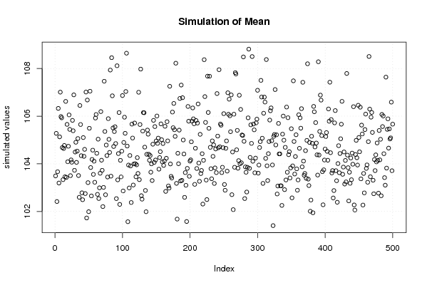
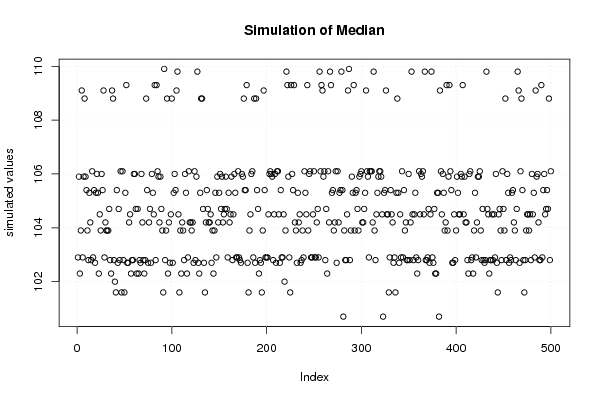
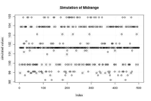
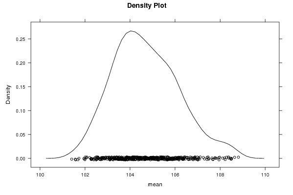
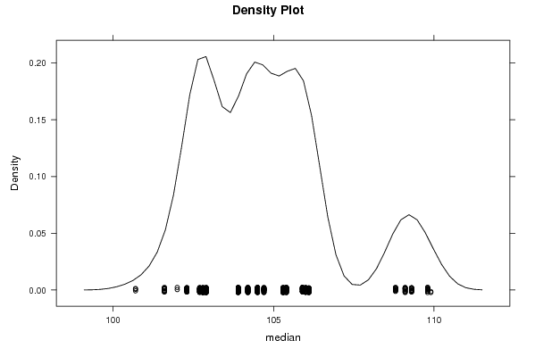
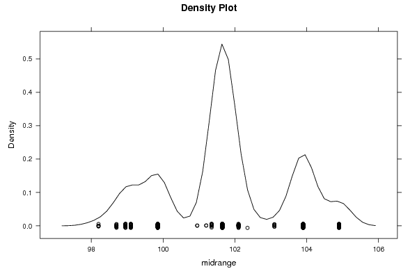
Figures (Output of Computation) | |||||||||||||||||||||||||||||||||||||||||||||||||||||||||||||||||||||||||||||||||
Input Parameters & R Code | |||||||||||||||||||||||||||||||||||||||||||||||||||||||||||||||||||||||||||||||||
| Parameters (Session): | |||||||||||||||||||||||||||||||||||||||||||||||||||||||||||||||||||||||||||||||||
| par1 = 500 ; par2 = 12 ; | |||||||||||||||||||||||||||||||||||||||||||||||||||||||||||||||||||||||||||||||||
| Parameters (R input): | |||||||||||||||||||||||||||||||||||||||||||||||||||||||||||||||||||||||||||||||||
| par1 = 500 ; par2 = 12 ; | |||||||||||||||||||||||||||||||||||||||||||||||||||||||||||||||||||||||||||||||||
| R code (references can be found in the software module): | |||||||||||||||||||||||||||||||||||||||||||||||||||||||||||||||||||||||||||||||||
par1 <- as.numeric(par1) | |||||||||||||||||||||||||||||||||||||||||||||||||||||||||||||||||||||||||||||||||