Repository of Reproducible Computations

Free Statistics

of Irreproducible Research!

Author's title

Author

*Unverified author*

R Software Module

rwasp_autocorrelation.wasp

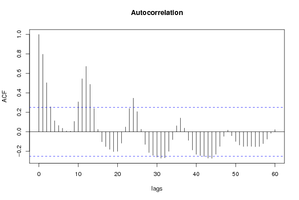
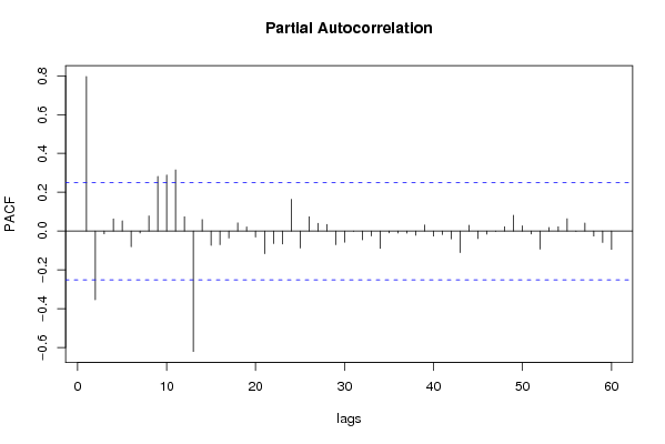
Title produced by software

(Partial) Autocorrelation Function

Date of computation

Sun, 14 Dec 2008 09:25:08 -0700

Cite this page as follows

Statistical Computations at FreeStatistics.org, Office for Research Development and Education, URL https://freestatistics.org/blog/index.php?v=date/2008/Dec/14/t12292719395z9b4nheyq3xc97.htm/, Retrieved Thu, 16 May 2024 02:09:25 +0000

Statistical Computations at FreeStatistics.org, Office for Research Development and Education, URL https://freestatistics.org/blog/index.php?pk=33464, Retrieved Thu, 16 May 2024 02:09:25 +0000

QR Codes:

Paste this QR Code to cite your computation.

Original text written by user:

IsPrivate?

No (this computation is public)

User-defined keywords

Estimated Impact

168

Family? (F = Feedback message, R = changed R code, M = changed R Module, P = changed Parameters, D = changed Data)

-       [(Partial) Autocorrelation Function] [paper autocorrela...] [2008-12-14 16:25:08] [4940af498c7c54f3992f17142bd40069] [Current]
-   P     [(Partial) Autocorrelation Function] [paper autocorrela...] [2008-12-14 16:31:59] [85134b6edb9973b9193450dd2306c65b] 
-   P       [(Partial) Autocorrelation Function] [paper autocorrela...] [2008-12-14 16:35:41] [85134b6edb9973b9193450dd2306c65b] 
- RMP       [Spectral Analysis] [paper spectrale a...] [2008-12-14 16:40:55] [85134b6edb9973b9193450dd2306c65b] 
-   P         [Spectral Analysis] [paper spectrale a...] [2008-12-14 16:47:07] [85134b6edb9973b9193450dd2306c65b] 
-   P           [Spectral Analysis] [paper spectrale a...] [2008-12-14 16:53:15] [85134b6edb9973b9193450dd2306c65b] 
- RMP           [ARIMA Backward Selection] [paper arima backw...] [2008-12-14 17:10:44] [85134b6edb9973b9193450dd2306c65b] 

Feedback Forum

Post a new message

Dataseries X:

Download CSV

Histogram

Boxplots

Summary of computational transaction
Raw Input	view raw input (R code)
Raw Output	view raw output of R engine
Computing time	1 seconds
R Server	'Gwilym Jenkins' @ 72.249.127.135

\begin{tabular}{lllllllll}
\hline
Summary of computational transaction \tabularnewline
Raw Input & view raw input (R code)  \tabularnewline
Raw Output & view raw output of R engine  \tabularnewline
Computing time & 1 seconds \tabularnewline
R Server & 'Gwilym Jenkins' @ 72.249.127.135 \tabularnewline
\hline
\end{tabular}
%Source: https://freestatistics.org/blog/index.php?pk=33464&T=0

[TABLE]
[ROW][C]Summary of computational transaction[/C][/ROW]
[ROW][C]Raw Input[/C][C]view raw input (R code) [/C][/ROW]
[ROW][C]Raw Output[/C][C]view raw output of R engine [/C][/ROW]
[ROW][C]Computing time[/C][C]1 seconds[/C][/ROW]
[ROW][C]R Server[/C][C]'Gwilym Jenkins' @ 72.249.127.135[/C][/ROW]
[/TABLE]
Source: https://freestatistics.org/blog/index.php?pk=33464&T=0

Globally Unique Identifier (entire table): ba.freestatistics.org/blog/index.php?pk=33464&T=0

As an alternative you can also use a QR Code:

The GUIDs for individual cells are displayed in the table below:

Summary of computational transaction
Raw Input	view raw input (R code)
Raw Output	view raw output of R engine
Computing time	1 seconds
R Server	'Gwilym Jenkins' @ 72.249.127.135

Autocorrelation Function
Time lag k	ACF(k)	T-STAT	P-value
1	0.796303	6.2193	0
2	0.504403	3.9395	0.000106
3	0.257119	2.0082	0.02453
4	0.113478	0.8863	0.189471
5	0.065547	0.5119	0.305271
6	0.037089	0.2897	0.386525
7	0.008891	0.0694	0.472432
8	0.007034	0.0549	0.478183
9	0.107694	0.8411	0.201784
10	0.307819	2.4041	0.009631
11	0.54495	4.2562	3.6e-05
12	0.672194	5.25	1e-06
13	0.487675	3.8089	0.000163
14	0.23919	1.8681	0.033274
15	0.024647	0.1925	0.423997
16	-0.102473	-0.8003	0.21331
17	-0.151729	-1.185	0.120298
18	-0.179994	-1.4058	0.082428
19	-0.203336	-1.5881	0.058717
20	-0.200574	-1.5665	0.061198
21	-0.116105	-0.9068	0.184037
22	0.050212	0.3922	0.348149
23	0.239263	1.8687	0.033234
24	0.346087	2.703	0.004444
25	0.207598	1.6214	0.055046
26	0.026045	0.2034	0.419742
27	-0.129081	-1.0082	0.158682
28	-0.212618	-1.6606	0.050963
29	-0.241607	-1.887	0.03196
30	-0.259839	-2.0294	0.023393
31	-0.270359	-2.1116	0.019414
32	-0.267237	-2.0872	0.020528
33	-0.200469	-1.5657	0.061295
34	-0.080245	-0.6267	0.266586
35	0.061835	0.4829	0.31543
36	0.142055	1.1095	0.135788
37	0.038586	0.3014	0.382081
38	-0.087484	-0.6833	0.248512
39	-0.186189	-1.4542	0.075511
40	-0.231389	-1.8072	0.037831
41	-0.244362	-1.9085	0.030516
42	-0.252631	-1.9731	0.026509
43	-0.26962	-2.1058	0.019673
44	-0.272166	-2.1257	0.018793
45	-0.23061	-1.8011	0.038314
46	-0.149725	-1.1694	0.123398
47	-0.046092	-0.36	0.36005
48	0.01775	0.1386	0.445098
49	-0.040605	-0.3171	0.376113
50	-0.099223	-0.775	0.22068
51	-0.135585	-1.059	0.146898
52	-0.15087	-1.1783	0.12162
53	-0.148691	-1.1613	0.12502
54	-0.149724	-1.1694	0.123399
55	-0.153131	-1.196	0.118164
56	-0.150225	-1.1733	0.122619
57	-0.121361	-0.9479	0.17347
58	-0.075424	-0.5891	0.278992
59	-0.014772	-0.1154	0.454265
60	0.022081	0.1725	0.431825

\begin{tabular}{lllllllll}
\hline
Autocorrelation Function \tabularnewline
Time lag k & ACF(k) & T-STAT & P-value \tabularnewline
1 & 0.796303 & 6.2193 & 0 \tabularnewline
2 & 0.504403 & 3.9395 & 0.000106 \tabularnewline
3 & 0.257119 & 2.0082 & 0.02453 \tabularnewline
4 & 0.113478 & 0.8863 & 0.189471 \tabularnewline
5 & 0.065547 & 0.5119 & 0.305271 \tabularnewline
6 & 0.037089 & 0.2897 & 0.386525 \tabularnewline
7 & 0.008891 & 0.0694 & 0.472432 \tabularnewline
8 & 0.007034 & 0.0549 & 0.478183 \tabularnewline
9 & 0.107694 & 0.8411 & 0.201784 \tabularnewline
10 & 0.307819 & 2.4041 & 0.009631 \tabularnewline
11 & 0.54495 & 4.2562 & 3.6e-05 \tabularnewline
12 & 0.672194 & 5.25 & 1e-06 \tabularnewline
13 & 0.487675 & 3.8089 & 0.000163 \tabularnewline
14 & 0.23919 & 1.8681 & 0.033274 \tabularnewline
15 & 0.024647 & 0.1925 & 0.423997 \tabularnewline
16 & -0.102473 & -0.8003 & 0.21331 \tabularnewline
17 & -0.151729 & -1.185 & 0.120298 \tabularnewline
18 & -0.179994 & -1.4058 & 0.082428 \tabularnewline
19 & -0.203336 & -1.5881 & 0.058717 \tabularnewline
20 & -0.200574 & -1.5665 & 0.061198 \tabularnewline
21 & -0.116105 & -0.9068 & 0.184037 \tabularnewline
22 & 0.050212 & 0.3922 & 0.348149 \tabularnewline
23 & 0.239263 & 1.8687 & 0.033234 \tabularnewline
24 & 0.346087 & 2.703 & 0.004444 \tabularnewline
25 & 0.207598 & 1.6214 & 0.055046 \tabularnewline
26 & 0.026045 & 0.2034 & 0.419742 \tabularnewline
27 & -0.129081 & -1.0082 & 0.158682 \tabularnewline
28 & -0.212618 & -1.6606 & 0.050963 \tabularnewline
29 & -0.241607 & -1.887 & 0.03196 \tabularnewline
30 & -0.259839 & -2.0294 & 0.023393 \tabularnewline
31 & -0.270359 & -2.1116 & 0.019414 \tabularnewline
32 & -0.267237 & -2.0872 & 0.020528 \tabularnewline
33 & -0.200469 & -1.5657 & 0.061295 \tabularnewline
34 & -0.080245 & -0.6267 & 0.266586 \tabularnewline
35 & 0.061835 & 0.4829 & 0.31543 \tabularnewline
36 & 0.142055 & 1.1095 & 0.135788 \tabularnewline
37 & 0.038586 & 0.3014 & 0.382081 \tabularnewline
38 & -0.087484 & -0.6833 & 0.248512 \tabularnewline
39 & -0.186189 & -1.4542 & 0.075511 \tabularnewline
40 & -0.231389 & -1.8072 & 0.037831 \tabularnewline
41 & -0.244362 & -1.9085 & 0.030516 \tabularnewline
42 & -0.252631 & -1.9731 & 0.026509 \tabularnewline
43 & -0.26962 & -2.1058 & 0.019673 \tabularnewline
44 & -0.272166 & -2.1257 & 0.018793 \tabularnewline
45 & -0.23061 & -1.8011 & 0.038314 \tabularnewline
46 & -0.149725 & -1.1694 & 0.123398 \tabularnewline
47 & -0.046092 & -0.36 & 0.36005 \tabularnewline
48 & 0.01775 & 0.1386 & 0.445098 \tabularnewline
49 & -0.040605 & -0.3171 & 0.376113 \tabularnewline
50 & -0.099223 & -0.775 & 0.22068 \tabularnewline
51 & -0.135585 & -1.059 & 0.146898 \tabularnewline
52 & -0.15087 & -1.1783 & 0.12162 \tabularnewline
53 & -0.148691 & -1.1613 & 0.12502 \tabularnewline
54 & -0.149724 & -1.1694 & 0.123399 \tabularnewline
55 & -0.153131 & -1.196 & 0.118164 \tabularnewline
56 & -0.150225 & -1.1733 & 0.122619 \tabularnewline
57 & -0.121361 & -0.9479 & 0.17347 \tabularnewline
58 & -0.075424 & -0.5891 & 0.278992 \tabularnewline
59 & -0.014772 & -0.1154 & 0.454265 \tabularnewline
60 & 0.022081 & 0.1725 & 0.431825 \tabularnewline
\hline
\end{tabular}
%Source: https://freestatistics.org/blog/index.php?pk=33464&T=1

[TABLE]
[ROW][C]Autocorrelation Function[/C][/ROW]
[ROW][C]Time lag k[/C][C]ACF(k)[/C][C]T-STAT[/C][C]P-value[/C][/ROW]
[ROW][C]1[/C][C]0.796303[/C][C]6.2193[/C][C]0[/C][/ROW]
[ROW][C]2[/C][C]0.504403[/C][C]3.9395[/C][C]0.000106[/C][/ROW]
[ROW][C]3[/C][C]0.257119[/C][C]2.0082[/C][C]0.02453[/C][/ROW]
[ROW][C]4[/C][C]0.113478[/C][C]0.8863[/C][C]0.189471[/C][/ROW]
[ROW][C]5[/C][C]0.065547[/C][C]0.5119[/C][C]0.305271[/C][/ROW]
[ROW][C]6[/C][C]0.037089[/C][C]0.2897[/C][C]0.386525[/C][/ROW]
[ROW][C]7[/C][C]0.008891[/C][C]0.0694[/C][C]0.472432[/C][/ROW]
[ROW][C]8[/C][C]0.007034[/C][C]0.0549[/C][C]0.478183[/C][/ROW]
[ROW][C]9[/C][C]0.107694[/C][C]0.8411[/C][C]0.201784[/C][/ROW]
[ROW][C]10[/C][C]0.307819[/C][C]2.4041[/C][C]0.009631[/C][/ROW]
[ROW][C]11[/C][C]0.54495[/C][C]4.2562[/C][C]3.6e-05[/C][/ROW]
[ROW][C]12[/C][C]0.672194[/C][C]5.25[/C][C]1e-06[/C][/ROW]
[ROW][C]13[/C][C]0.487675[/C][C]3.8089[/C][C]0.000163[/C][/ROW]
[ROW][C]14[/C][C]0.23919[/C][C]1.8681[/C][C]0.033274[/C][/ROW]
[ROW][C]15[/C][C]0.024647[/C][C]0.1925[/C][C]0.423997[/C][/ROW]
[ROW][C]16[/C][C]-0.102473[/C][C]-0.8003[/C][C]0.21331[/C][/ROW]
[ROW][C]17[/C][C]-0.151729[/C][C]-1.185[/C][C]0.120298[/C][/ROW]
[ROW][C]18[/C][C]-0.179994[/C][C]-1.4058[/C][C]0.082428[/C][/ROW]
[ROW][C]19[/C][C]-0.203336[/C][C]-1.5881[/C][C]0.058717[/C][/ROW]
[ROW][C]20[/C][C]-0.200574[/C][C]-1.5665[/C][C]0.061198[/C][/ROW]
[ROW][C]21[/C][C]-0.116105[/C][C]-0.9068[/C][C]0.184037[/C][/ROW]
[ROW][C]22[/C][C]0.050212[/C][C]0.3922[/C][C]0.348149[/C][/ROW]
[ROW][C]23[/C][C]0.239263[/C][C]1.8687[/C][C]0.033234[/C][/ROW]
[ROW][C]24[/C][C]0.346087[/C][C]2.703[/C][C]0.004444[/C][/ROW]
[ROW][C]25[/C][C]0.207598[/C][C]1.6214[/C][C]0.055046[/C][/ROW]
[ROW][C]26[/C][C]0.026045[/C][C]0.2034[/C][C]0.419742[/C][/ROW]
[ROW][C]27[/C][C]-0.129081[/C][C]-1.0082[/C][C]0.158682[/C][/ROW]
[ROW][C]28[/C][C]-0.212618[/C][C]-1.6606[/C][C]0.050963[/C][/ROW]
[ROW][C]29[/C][C]-0.241607[/C][C]-1.887[/C][C]0.03196[/C][/ROW]
[ROW][C]30[/C][C]-0.259839[/C][C]-2.0294[/C][C]0.023393[/C][/ROW]
[ROW][C]31[/C][C]-0.270359[/C][C]-2.1116[/C][C]0.019414[/C][/ROW]
[ROW][C]32[/C][C]-0.267237[/C][C]-2.0872[/C][C]0.020528[/C][/ROW]
[ROW][C]33[/C][C]-0.200469[/C][C]-1.5657[/C][C]0.061295[/C][/ROW]
[ROW][C]34[/C][C]-0.080245[/C][C]-0.6267[/C][C]0.266586[/C][/ROW]
[ROW][C]35[/C][C]0.061835[/C][C]0.4829[/C][C]0.31543[/C][/ROW]
[ROW][C]36[/C][C]0.142055[/C][C]1.1095[/C][C]0.135788[/C][/ROW]
[ROW][C]37[/C][C]0.038586[/C][C]0.3014[/C][C]0.382081[/C][/ROW]
[ROW][C]38[/C][C]-0.087484[/C][C]-0.6833[/C][C]0.248512[/C][/ROW]
[ROW][C]39[/C][C]-0.186189[/C][C]-1.4542[/C][C]0.075511[/C][/ROW]
[ROW][C]40[/C][C]-0.231389[/C][C]-1.8072[/C][C]0.037831[/C][/ROW]
[ROW][C]41[/C][C]-0.244362[/C][C]-1.9085[/C][C]0.030516[/C][/ROW]
[ROW][C]42[/C][C]-0.252631[/C][C]-1.9731[/C][C]0.026509[/C][/ROW]
[ROW][C]43[/C][C]-0.26962[/C][C]-2.1058[/C][C]0.019673[/C][/ROW]
[ROW][C]44[/C][C]-0.272166[/C][C]-2.1257[/C][C]0.018793[/C][/ROW]
[ROW][C]45[/C][C]-0.23061[/C][C]-1.8011[/C][C]0.038314[/C][/ROW]
[ROW][C]46[/C][C]-0.149725[/C][C]-1.1694[/C][C]0.123398[/C][/ROW]
[ROW][C]47[/C][C]-0.046092[/C][C]-0.36[/C][C]0.36005[/C][/ROW]
[ROW][C]48[/C][C]0.01775[/C][C]0.1386[/C][C]0.445098[/C][/ROW]
[ROW][C]49[/C][C]-0.040605[/C][C]-0.3171[/C][C]0.376113[/C][/ROW]
[ROW][C]50[/C][C]-0.099223[/C][C]-0.775[/C][C]0.22068[/C][/ROW]
[ROW][C]51[/C][C]-0.135585[/C][C]-1.059[/C][C]0.146898[/C][/ROW]
[ROW][C]52[/C][C]-0.15087[/C][C]-1.1783[/C][C]0.12162[/C][/ROW]
[ROW][C]53[/C][C]-0.148691[/C][C]-1.1613[/C][C]0.12502[/C][/ROW]
[ROW][C]54[/C][C]-0.149724[/C][C]-1.1694[/C][C]0.123399[/C][/ROW]
[ROW][C]55[/C][C]-0.153131[/C][C]-1.196[/C][C]0.118164[/C][/ROW]
[ROW][C]56[/C][C]-0.150225[/C][C]-1.1733[/C][C]0.122619[/C][/ROW]
[ROW][C]57[/C][C]-0.121361[/C][C]-0.9479[/C][C]0.17347[/C][/ROW]
[ROW][C]58[/C][C]-0.075424[/C][C]-0.5891[/C][C]0.278992[/C][/ROW]
[ROW][C]59[/C][C]-0.014772[/C][C]-0.1154[/C][C]0.454265[/C][/ROW]
[ROW][C]60[/C][C]0.022081[/C][C]0.1725[/C][C]0.431825[/C][/ROW]
[/TABLE]
Source: https://freestatistics.org/blog/index.php?pk=33464&T=1

Globally Unique Identifier (entire table): ba.freestatistics.org/blog/index.php?pk=33464&T=1

As an alternative you can also use a QR Code:

The GUIDs for individual cells are displayed in the table below:

Autocorrelation Function
Time lag k	ACF(k)	T-STAT	P-value
1	0.796303	6.2193	0
2	0.504403	3.9395	0.000106
3	0.257119	2.0082	0.02453
4	0.113478	0.8863	0.189471
5	0.065547	0.5119	0.305271
6	0.037089	0.2897	0.386525
7	0.008891	0.0694	0.472432
8	0.007034	0.0549	0.478183
9	0.107694	0.8411	0.201784
10	0.307819	2.4041	0.009631
11	0.54495	4.2562	3.6e-05
12	0.672194	5.25	1e-06
13	0.487675	3.8089	0.000163
14	0.23919	1.8681	0.033274
15	0.024647	0.1925	0.423997
16	-0.102473	-0.8003	0.21331
17	-0.151729	-1.185	0.120298
18	-0.179994	-1.4058	0.082428
19	-0.203336	-1.5881	0.058717
20	-0.200574	-1.5665	0.061198
21	-0.116105	-0.9068	0.184037
22	0.050212	0.3922	0.348149
23	0.239263	1.8687	0.033234
24	0.346087	2.703	0.004444
25	0.207598	1.6214	0.055046
26	0.026045	0.2034	0.419742
27	-0.129081	-1.0082	0.158682
28	-0.212618	-1.6606	0.050963
29	-0.241607	-1.887	0.03196
30	-0.259839	-2.0294	0.023393
31	-0.270359	-2.1116	0.019414
32	-0.267237	-2.0872	0.020528
33	-0.200469	-1.5657	0.061295
34	-0.080245	-0.6267	0.266586
35	0.061835	0.4829	0.31543
36	0.142055	1.1095	0.135788
37	0.038586	0.3014	0.382081
38	-0.087484	-0.6833	0.248512
39	-0.186189	-1.4542	0.075511
40	-0.231389	-1.8072	0.037831
41	-0.244362	-1.9085	0.030516
42	-0.252631	-1.9731	0.026509
43	-0.26962	-2.1058	0.019673
44	-0.272166	-2.1257	0.018793
45	-0.23061	-1.8011	0.038314
46	-0.149725	-1.1694	0.123398
47	-0.046092	-0.36	0.36005
48	0.01775	0.1386	0.445098
49	-0.040605	-0.3171	0.376113
50	-0.099223	-0.775	0.22068
51	-0.135585	-1.059	0.146898
52	-0.15087	-1.1783	0.12162
53	-0.148691	-1.1613	0.12502
54	-0.149724	-1.1694	0.123399
55	-0.153131	-1.196	0.118164
56	-0.150225	-1.1733	0.122619
57	-0.121361	-0.9479	0.17347
58	-0.075424	-0.5891	0.278992
59	-0.014772	-0.1154	0.454265
60	0.022081	0.1725	0.431825

Partial Autocorrelation Function
Time lag k	PACF(k)	T-STAT	P-value
1	0.796303	6.2193	0
2	-0.354456	-2.7684	0.003725
3	-0.014549	-0.1136	0.454953
4	0.062354	0.487	0.314002
5	0.052585	0.4107	0.341366
6	-0.080978	-0.6325	0.264725
7	-0.010473	-0.0818	0.467539
8	0.077496	0.6053	0.273626
9	0.281482	2.1984	0.01586
10	0.288956	2.2568	0.013807
11	0.315343	2.4629	0.00831
12	0.07306	0.5706	0.285178
13	-0.62076	-4.8483	4e-06
14	0.058975	0.4606	0.323357
15	-0.073599	-0.5748	0.283761
16	-0.069981	-0.5466	0.293335
17	-0.035655	-0.2785	0.390795
18	0.041837	0.3268	0.372485
19	0.021081	0.1646	0.434882
20	-0.031113	-0.243	0.404411
21	-0.116836	-0.9125	0.182544
22	-0.064468	-0.5035	0.30821
23	-0.066499	-0.5194	0.302689
24	0.163427	1.2764	0.103325
25	-0.08724	-0.6814	0.24911
26	0.07306	0.5706	0.285178
27	0.039657	0.3097	0.378911
28	0.034334	0.2682	0.394743
29	-0.070315	-0.5492	0.292444
30	-0.057364	-0.448	0.327862
31	-0.000824	-0.0064	0.497443
32	-0.045634	-0.3564	0.361381
33	-0.02543	-0.1986	0.421612
34	-0.089426	-0.6984	0.243779
35	-0.009765	-0.0763	0.469729
36	-0.010266	-0.0802	0.468179
37	-0.011044	-0.0863	0.465772
38	-0.021683	-0.1693	0.433042
39	0.031228	0.2439	0.404063
40	-0.026335	-0.2057	0.418861
41	-0.017873	-0.1396	0.444721
42	-0.040395	-0.3155	0.376732
43	-0.111343	-0.8696	0.193959
44	0.02948	0.2302	0.409335
45	-0.039217	-0.3063	0.380211
46	-0.016052	-0.1254	0.450323
47	-0.0015	-0.0117	0.495347
48	0.021632	0.169	0.433196
49	0.081137	0.6337	0.264322
50	0.02709	0.2116	0.416571
51	-0.015402	-0.1203	0.452324
52	-0.092874	-0.7254	0.2355
53	0.018397	0.1437	0.44311
54	0.021558	0.1684	0.433422
55	0.063198	0.4936	0.311683
56	-0.001964	-0.0153	0.493904
57	0.041297	0.3225	0.374074
58	-0.025888	-0.2022	0.420218
59	-0.058872	-0.4598	0.323646
60	-0.094839	-0.7407	0.230854

\begin{tabular}{lllllllll}
\hline
Partial Autocorrelation Function \tabularnewline
Time lag k & PACF(k) & T-STAT & P-value \tabularnewline
1 & 0.796303 & 6.2193 & 0 \tabularnewline
2 & -0.354456 & -2.7684 & 0.003725 \tabularnewline
3 & -0.014549 & -0.1136 & 0.454953 \tabularnewline
4 & 0.062354 & 0.487 & 0.314002 \tabularnewline
5 & 0.052585 & 0.4107 & 0.341366 \tabularnewline
6 & -0.080978 & -0.6325 & 0.264725 \tabularnewline
7 & -0.010473 & -0.0818 & 0.467539 \tabularnewline
8 & 0.077496 & 0.6053 & 0.273626 \tabularnewline
9 & 0.281482 & 2.1984 & 0.01586 \tabularnewline
10 & 0.288956 & 2.2568 & 0.013807 \tabularnewline
11 & 0.315343 & 2.4629 & 0.00831 \tabularnewline
12 & 0.07306 & 0.5706 & 0.285178 \tabularnewline
13 & -0.62076 & -4.8483 & 4e-06 \tabularnewline
14 & 0.058975 & 0.4606 & 0.323357 \tabularnewline
15 & -0.073599 & -0.5748 & 0.283761 \tabularnewline
16 & -0.069981 & -0.5466 & 0.293335 \tabularnewline
17 & -0.035655 & -0.2785 & 0.390795 \tabularnewline
18 & 0.041837 & 0.3268 & 0.372485 \tabularnewline
19 & 0.021081 & 0.1646 & 0.434882 \tabularnewline
20 & -0.031113 & -0.243 & 0.404411 \tabularnewline
21 & -0.116836 & -0.9125 & 0.182544 \tabularnewline
22 & -0.064468 & -0.5035 & 0.30821 \tabularnewline
23 & -0.066499 & -0.5194 & 0.302689 \tabularnewline
24 & 0.163427 & 1.2764 & 0.103325 \tabularnewline
25 & -0.08724 & -0.6814 & 0.24911 \tabularnewline
26 & 0.07306 & 0.5706 & 0.285178 \tabularnewline
27 & 0.039657 & 0.3097 & 0.378911 \tabularnewline
28 & 0.034334 & 0.2682 & 0.394743 \tabularnewline
29 & -0.070315 & -0.5492 & 0.292444 \tabularnewline
30 & -0.057364 & -0.448 & 0.327862 \tabularnewline
31 & -0.000824 & -0.0064 & 0.497443 \tabularnewline
32 & -0.045634 & -0.3564 & 0.361381 \tabularnewline
33 & -0.02543 & -0.1986 & 0.421612 \tabularnewline
34 & -0.089426 & -0.6984 & 0.243779 \tabularnewline
35 & -0.009765 & -0.0763 & 0.469729 \tabularnewline
36 & -0.010266 & -0.0802 & 0.468179 \tabularnewline
37 & -0.011044 & -0.0863 & 0.465772 \tabularnewline
38 & -0.021683 & -0.1693 & 0.433042 \tabularnewline
39 & 0.031228 & 0.2439 & 0.404063 \tabularnewline
40 & -0.026335 & -0.2057 & 0.418861 \tabularnewline
41 & -0.017873 & -0.1396 & 0.444721 \tabularnewline
42 & -0.040395 & -0.3155 & 0.376732 \tabularnewline
43 & -0.111343 & -0.8696 & 0.193959 \tabularnewline
44 & 0.02948 & 0.2302 & 0.409335 \tabularnewline
45 & -0.039217 & -0.3063 & 0.380211 \tabularnewline
46 & -0.016052 & -0.1254 & 0.450323 \tabularnewline
47 & -0.0015 & -0.0117 & 0.495347 \tabularnewline
48 & 0.021632 & 0.169 & 0.433196 \tabularnewline
49 & 0.081137 & 0.6337 & 0.264322 \tabularnewline
50 & 0.02709 & 0.2116 & 0.416571 \tabularnewline
51 & -0.015402 & -0.1203 & 0.452324 \tabularnewline
52 & -0.092874 & -0.7254 & 0.2355 \tabularnewline
53 & 0.018397 & 0.1437 & 0.44311 \tabularnewline
54 & 0.021558 & 0.1684 & 0.433422 \tabularnewline
55 & 0.063198 & 0.4936 & 0.311683 \tabularnewline
56 & -0.001964 & -0.0153 & 0.493904 \tabularnewline
57 & 0.041297 & 0.3225 & 0.374074 \tabularnewline
58 & -0.025888 & -0.2022 & 0.420218 \tabularnewline
59 & -0.058872 & -0.4598 & 0.323646 \tabularnewline
60 & -0.094839 & -0.7407 & 0.230854 \tabularnewline
\hline
\end{tabular}
%Source: https://freestatistics.org/blog/index.php?pk=33464&T=2

[TABLE]
[ROW][C]Partial Autocorrelation Function[/C][/ROW]
[ROW][C]Time lag k[/C][C]PACF(k)[/C][C]T-STAT[/C][C]P-value[/C][/ROW]
[ROW][C]1[/C][C]0.796303[/C][C]6.2193[/C][C]0[/C][/ROW]
[ROW][C]2[/C][C]-0.354456[/C][C]-2.7684[/C][C]0.003725[/C][/ROW]
[ROW][C]3[/C][C]-0.014549[/C][C]-0.1136[/C][C]0.454953[/C][/ROW]
[ROW][C]4[/C][C]0.062354[/C][C]0.487[/C][C]0.314002[/C][/ROW]
[ROW][C]5[/C][C]0.052585[/C][C]0.4107[/C][C]0.341366[/C][/ROW]
[ROW][C]6[/C][C]-0.080978[/C][C]-0.6325[/C][C]0.264725[/C][/ROW]
[ROW][C]7[/C][C]-0.010473[/C][C]-0.0818[/C][C]0.467539[/C][/ROW]
[ROW][C]8[/C][C]0.077496[/C][C]0.6053[/C][C]0.273626[/C][/ROW]
[ROW][C]9[/C][C]0.281482[/C][C]2.1984[/C][C]0.01586[/C][/ROW]
[ROW][C]10[/C][C]0.288956[/C][C]2.2568[/C][C]0.013807[/C][/ROW]
[ROW][C]11[/C][C]0.315343[/C][C]2.4629[/C][C]0.00831[/C][/ROW]
[ROW][C]12[/C][C]0.07306[/C][C]0.5706[/C][C]0.285178[/C][/ROW]
[ROW][C]13[/C][C]-0.62076[/C][C]-4.8483[/C][C]4e-06[/C][/ROW]
[ROW][C]14[/C][C]0.058975[/C][C]0.4606[/C][C]0.323357[/C][/ROW]
[ROW][C]15[/C][C]-0.073599[/C][C]-0.5748[/C][C]0.283761[/C][/ROW]
[ROW][C]16[/C][C]-0.069981[/C][C]-0.5466[/C][C]0.293335[/C][/ROW]
[ROW][C]17[/C][C]-0.035655[/C][C]-0.2785[/C][C]0.390795[/C][/ROW]
[ROW][C]18[/C][C]0.041837[/C][C]0.3268[/C][C]0.372485[/C][/ROW]
[ROW][C]19[/C][C]0.021081[/C][C]0.1646[/C][C]0.434882[/C][/ROW]
[ROW][C]20[/C][C]-0.031113[/C][C]-0.243[/C][C]0.404411[/C][/ROW]
[ROW][C]21[/C][C]-0.116836[/C][C]-0.9125[/C][C]0.182544[/C][/ROW]
[ROW][C]22[/C][C]-0.064468[/C][C]-0.5035[/C][C]0.30821[/C][/ROW]
[ROW][C]23[/C][C]-0.066499[/C][C]-0.5194[/C][C]0.302689[/C][/ROW]
[ROW][C]24[/C][C]0.163427[/C][C]1.2764[/C][C]0.103325[/C][/ROW]
[ROW][C]25[/C][C]-0.08724[/C][C]-0.6814[/C][C]0.24911[/C][/ROW]
[ROW][C]26[/C][C]0.07306[/C][C]0.5706[/C][C]0.285178[/C][/ROW]
[ROW][C]27[/C][C]0.039657[/C][C]0.3097[/C][C]0.378911[/C][/ROW]
[ROW][C]28[/C][C]0.034334[/C][C]0.2682[/C][C]0.394743[/C][/ROW]
[ROW][C]29[/C][C]-0.070315[/C][C]-0.5492[/C][C]0.292444[/C][/ROW]
[ROW][C]30[/C][C]-0.057364[/C][C]-0.448[/C][C]0.327862[/C][/ROW]
[ROW][C]31[/C][C]-0.000824[/C][C]-0.0064[/C][C]0.497443[/C][/ROW]
[ROW][C]32[/C][C]-0.045634[/C][C]-0.3564[/C][C]0.361381[/C][/ROW]
[ROW][C]33[/C][C]-0.02543[/C][C]-0.1986[/C][C]0.421612[/C][/ROW]
[ROW][C]34[/C][C]-0.089426[/C][C]-0.6984[/C][C]0.243779[/C][/ROW]
[ROW][C]35[/C][C]-0.009765[/C][C]-0.0763[/C][C]0.469729[/C][/ROW]
[ROW][C]36[/C][C]-0.010266[/C][C]-0.0802[/C][C]0.468179[/C][/ROW]
[ROW][C]37[/C][C]-0.011044[/C][C]-0.0863[/C][C]0.465772[/C][/ROW]
[ROW][C]38[/C][C]-0.021683[/C][C]-0.1693[/C][C]0.433042[/C][/ROW]
[ROW][C]39[/C][C]0.031228[/C][C]0.2439[/C][C]0.404063[/C][/ROW]
[ROW][C]40[/C][C]-0.026335[/C][C]-0.2057[/C][C]0.418861[/C][/ROW]
[ROW][C]41[/C][C]-0.017873[/C][C]-0.1396[/C][C]0.444721[/C][/ROW]
[ROW][C]42[/C][C]-0.040395[/C][C]-0.3155[/C][C]0.376732[/C][/ROW]
[ROW][C]43[/C][C]-0.111343[/C][C]-0.8696[/C][C]0.193959[/C][/ROW]
[ROW][C]44[/C][C]0.02948[/C][C]0.2302[/C][C]0.409335[/C][/ROW]
[ROW][C]45[/C][C]-0.039217[/C][C]-0.3063[/C][C]0.380211[/C][/ROW]
[ROW][C]46[/C][C]-0.016052[/C][C]-0.1254[/C][C]0.450323[/C][/ROW]
[ROW][C]47[/C][C]-0.0015[/C][C]-0.0117[/C][C]0.495347[/C][/ROW]
[ROW][C]48[/C][C]0.021632[/C][C]0.169[/C][C]0.433196[/C][/ROW]
[ROW][C]49[/C][C]0.081137[/C][C]0.6337[/C][C]0.264322[/C][/ROW]
[ROW][C]50[/C][C]0.02709[/C][C]0.2116[/C][C]0.416571[/C][/ROW]
[ROW][C]51[/C][C]-0.015402[/C][C]-0.1203[/C][C]0.452324[/C][/ROW]
[ROW][C]52[/C][C]-0.092874[/C][C]-0.7254[/C][C]0.2355[/C][/ROW]
[ROW][C]53[/C][C]0.018397[/C][C]0.1437[/C][C]0.44311[/C][/ROW]
[ROW][C]54[/C][C]0.021558[/C][C]0.1684[/C][C]0.433422[/C][/ROW]
[ROW][C]55[/C][C]0.063198[/C][C]0.4936[/C][C]0.311683[/C][/ROW]
[ROW][C]56[/C][C]-0.001964[/C][C]-0.0153[/C][C]0.493904[/C][/ROW]
[ROW][C]57[/C][C]0.041297[/C][C]0.3225[/C][C]0.374074[/C][/ROW]
[ROW][C]58[/C][C]-0.025888[/C][C]-0.2022[/C][C]0.420218[/C][/ROW]
[ROW][C]59[/C][C]-0.058872[/C][C]-0.4598[/C][C]0.323646[/C][/ROW]
[ROW][C]60[/C][C]-0.094839[/C][C]-0.7407[/C][C]0.230854[/C][/ROW]
[/TABLE]
Source: https://freestatistics.org/blog/index.php?pk=33464&T=2

Globally Unique Identifier (entire table): ba.freestatistics.org/blog/index.php?pk=33464&T=2

As an alternative you can also use a QR Code:

The GUIDs for individual cells are displayed in the table below:

Partial Autocorrelation Function
Time lag k	PACF(k)	T-STAT	P-value
1	0.796303	6.2193	0
2	-0.354456	-2.7684	0.003725
3	-0.014549	-0.1136	0.454953
4	0.062354	0.487	0.314002
5	0.052585	0.4107	0.341366
6	-0.080978	-0.6325	0.264725
7	-0.010473	-0.0818	0.467539
8	0.077496	0.6053	0.273626
9	0.281482	2.1984	0.01586
10	0.288956	2.2568	0.013807
11	0.315343	2.4629	0.00831
12	0.07306	0.5706	0.285178
13	-0.62076	-4.8483	4e-06
14	0.058975	0.4606	0.323357
15	-0.073599	-0.5748	0.283761
16	-0.069981	-0.5466	0.293335
17	-0.035655	-0.2785	0.390795
18	0.041837	0.3268	0.372485
19	0.021081	0.1646	0.434882
20	-0.031113	-0.243	0.404411
21	-0.116836	-0.9125	0.182544
22	-0.064468	-0.5035	0.30821
23	-0.066499	-0.5194	0.302689
24	0.163427	1.2764	0.103325
25	-0.08724	-0.6814	0.24911
26	0.07306	0.5706	0.285178
27	0.039657	0.3097	0.378911
28	0.034334	0.2682	0.394743
29	-0.070315	-0.5492	0.292444
30	-0.057364	-0.448	0.327862
31	-0.000824	-0.0064	0.497443
32	-0.045634	-0.3564	0.361381
33	-0.02543	-0.1986	0.421612
34	-0.089426	-0.6984	0.243779
35	-0.009765	-0.0763	0.469729
36	-0.010266	-0.0802	0.468179
37	-0.011044	-0.0863	0.465772
38	-0.021683	-0.1693	0.433042
39	0.031228	0.2439	0.404063
40	-0.026335	-0.2057	0.418861
41	-0.017873	-0.1396	0.444721
42	-0.040395	-0.3155	0.376732
43	-0.111343	-0.8696	0.193959
44	0.02948	0.2302	0.409335
45	-0.039217	-0.3063	0.380211
46	-0.016052	-0.1254	0.450323
47	-0.0015	-0.0117	0.495347
48	0.021632	0.169	0.433196
49	0.081137	0.6337	0.264322
50	0.02709	0.2116	0.416571
51	-0.015402	-0.1203	0.452324
52	-0.092874	-0.7254	0.2355
53	0.018397	0.1437	0.44311
54	0.021558	0.1684	0.433422
55	0.063198	0.4936	0.311683
56	-0.001964	-0.0153	0.493904
57	0.041297	0.3225	0.374074
58	-0.025888	-0.2022	0.420218
59	-0.058872	-0.4598	0.323646
60	-0.094839	-0.7407	0.230854

Figure 1

PNG link

Postscript link

PDF link

Figure 2

PNG link

Postscript link

PDF link

Parameters (Session):

par1 = 60 ; par2 = 1 ; par3 = 0 ; par4 = 0 ; par5 = 12 ;

Parameters (R input):

par1 = 60 ; par2 = 1 ; par3 = 0 ; par4 = 0 ; par5 = 12 ;

R code (references can be found in the software module):

if (par1 == 'Default') {
par1 = 10*log10(length(x))
} else {
par1 <- as.numeric(par1)
}
par2 <- as.numeric(par2)
par3 <- as.numeric(par3)
par4 <- as.numeric(par4)
par5 <- as.numeric(par5)
if (par2 == 0) {
x <- log(x)
} else {
x <- (x ^ par2 - 1) / par2
}
if (par3 > 0) x <- diff(x,lag=1,difference=par3)
if (par4 > 0) x <- diff(x,lag=par5,difference=par4)
bitmap(file='pic1.png')
racf <- acf(x,par1,main='Autocorrelation',xlab='lags',ylab='ACF')
dev.off()
bitmap(file='pic2.png')
rpacf <- pacf(x,par1,main='Partial Autocorrelation',xlab='lags',ylab='PACF')
dev.off()
(myacf <- c(racf$acf))
(mypacf <- c(rpacf$acf))
lengthx <- length(x)
sqrtn <- sqrt(lengthx)
load(file='createtable')
a<-table.start()
a<-table.row.start(a)
a<-table.element(a,'Autocorrelation Function',4,TRUE)
a<-table.row.end(a)
a<-table.row.start(a)
a<-table.element(a,'Time lag k',header=TRUE)
a<-table.element(a,hyperlink('basics.htm','ACF(k)','click here for more information about the Autocorrelation Function'),header=TRUE)
a<-table.element(a,'T-STAT',header=TRUE)
a<-table.element(a,'P-value',header=TRUE)
a<-table.row.end(a)
for (i in 2:(par1+1)) {
a<-table.row.start(a)
a<-table.element(a,i-1,header=TRUE)
a<-table.element(a,round(myacf[i],6))
mytstat <- myacf[i]*sqrtn
a<-table.element(a,round(mytstat,4))
a<-table.element(a,round(1-pt(abs(mytstat),lengthx),6))
a<-table.row.end(a)
}
a<-table.end(a)
table.save(a,file='mytable.tab')
a<-table.start()
a<-table.row.start(a)
a<-table.element(a,'Partial Autocorrelation Function',4,TRUE)
a<-table.row.end(a)
a<-table.row.start(a)
a<-table.element(a,'Time lag k',header=TRUE)
a<-table.element(a,hyperlink('basics.htm','PACF(k)','click here for more information about the Partial Autocorrelation Function'),header=TRUE)
a<-table.element(a,'T-STAT',header=TRUE)
a<-table.element(a,'P-value',header=TRUE)
a<-table.row.end(a)
for (i in 1:par1) {
a<-table.row.start(a)
a<-table.element(a,i,header=TRUE)
a<-table.element(a,round(mypacf[i],6))
mytstat <- mypacf[i]*sqrtn
a<-table.element(a,round(mytstat,4))
a<-table.element(a,round(1-pt(abs(mytstat),lengthx),6))
a<-table.row.end(a)
}
a<-table.end(a)
table.save(a,file='mytable1.tab')

Free Statistics

Description of Statistical Computation

Tree of Dependent Computations

Dataset

Tables (Output of Computation)

Figures (Output of Computation)

Input Parameters & R Code